
Example 1: Regional Full Moment Tensor
Clone project
This setup is comprised of 20 seismic stations that are randomly distributed within distances of 40 to 1000 km compared to a reference event. We will explore the solution space of a Full Moment Tensor . To copy the Example (including the data) to a directory outside of the package source directory, please edit the model path (referred to as $beat_models now on) and execute:
cd /path/to/beat/data/examples/
beat clone FullMT /'model path'/FullMT --copy_data --datatypes=seismic
This will create a BEAT project directory named FullMT with a configuration file (config_geometry.yaml) and some synthetic example data (seismic_data.pkl). This directory is going to be referred to as $project_directory in the following.
Calculate Greens Functions
The station-event geometry determines the grid of Greens Functions (GFs) that will need to be calculated next.
Please open $project_directory/config_geometry.yaml with any text editor (e.g. vi) and search for store_superdir. Here, it is written for now /home/vasyurhm/BEATS/GF, which is an example path to the directory of Greens Functions. This path needs to be replaced with the path to where the GFs are supposed to be stored on your computer. This directory is referred to as the $GF_path in the rest of the text. It is strongly recommended to use a separate directory apart from the beat source directory and the $project_directory as the GF databases can become very large, depending on the problem! For real examples, the GF databases may require up to several Gigabyte of free disc space. For our example the database that we are going to create is only around 30 Megabyte.:
cd $beat_models
beat build_gfs FullMT --datatypes='seismic'
This will create an empty Greens Function store named AqabaMT_ak135_1.000Hz_0 in the $GF_path. Under $GF_path/AqabaMT_ak135_1.000Hz_0/config it is recommended to cross-check again the velocity model and the specifications of the store (open with any texteditor). Dependent on the case study there are crucial parameters that often need to be changed from the default values: the spatial grid dimensions, the sample rate and the wave phases (body waves and/or surface waves) to be calculated.
In the $project_path/config_geometry.yaml under seismic config we find the gf_config, which holds the major parameters for GF calculation:
gf_config: !beat.SeismicGFConfig
  store_superdir: /home/vasyurhm/BEATS/GF/
  reference_model_idx: 0
  n_variations: [0, 1]
  error_depth: 0.1
  error_velocities: 0.1
  depth_limit_variation: 600.0
  earth_model_name: ak135-f-average.m
  use_crust2: false
  replace_water: false
  custom_velocity_model: |2
        0.             5.51           3.1            2.6         1264.           600.
        7.2            5.51           3.1            2.6         1264.           600.
        7.2            6.23           3.6            2.8         1283.           600.
       21.64           6.23           3.6            2.8         1283.           600.
    mantle
       21.64           7.95           4.45           3.2         1449.           600.
  source_depth_min: 8.0
  source_depth_max: 8.0
  source_depth_spacing: 1.0
  source_distance_radius: 1000.0
  source_distance_spacing: 1.0
  nworkers: 4
  reference_location: !beat.heart.ReferenceLocation
    lat: 29.07
    lon: 34.73
    elevation: 0.0
    depth: 0.0
    station: AqabaMT
  code: qseis
  sample_rate: 1.0
  rm_gfs: true
Here we see that instead of the global velocity model ak135 a custom velocity model is going to be used for all the stations. Below are the grid definitions of the GFs. In this example the source depth grid is limited to one depth (8 km) to reduce calculation time. As we have stations up to a distance of 970km distance to the event, the distance grid is accordingly extending up to 1000km. These grid sampling parameters as well as the sample rate are of major importance for the overall optimization. How to adjust these parameters according to individual case studies is described here.
The nworkers variable defines the number of CPUs to use in parallel for the GF calculations. As these calculations may become very expensive and time-consuming it is of advantage to use as many CPUs as available. To be still able to navigate in your Operating System without crashing the system it is good to leave one CPU work-less. Please edit the nworkers parameter now!
For our use-case the grid specifications are fine for now.
The seismic phases for which the GFs are going to be calculated are defined under waveforms in the $project_directory/config_geometry.yaml there are
- !beat.WaveformFitConfig
  include: true
  name: any_P
  blacklist: []
  channels: [Z]
  filterer:
  - !beat.heart.Filter
    lower_corner: 0.01
    upper_corner: 0.1
    order: 3
  distances: [0.0, 9.0]
  interpolation: multilinear
  arrival_taper: !beat.heart.ArrivalTaper
    a: -20.0
    b: -10.0
    c: 250.0
    d: 270.0
In this case the GFs are going to be calculated for the P body waves. We can add additional WaveformFitConfig*(s) if we want to include more phases. Like in our case of a regional setup we would like to include surface waves. For the build_GFs command only the existence of the *WaveformFitConfig and the name are of importance and we can ignore the other parameters so far. So lets add to the $project_directory/config_geometry.yaml file, the following config. Please copy ..
- !beat.WaveformFitConfig
  include: true
  name: slowest
  blacklist: []
  channels: [Z]
  filterer:
  - !beat.heart.Filter
    lower_corner: 0.001
    upper_corner: 0.1
    order: 4
  distances: [30.0, 90.0]
  interpolation: multilinear
  arrival_taper: !beat.heart.ArrivalTaper
    a: -15.0
    b: -10.0
    c: 50.0
    d: 55.0
and paste it below the ‘any_P’ WaveformFitConfig. Note: You should be having 2 WaveformFitConfig entries and both entries MUST have the same indentation! Your seismic_config within the $project_directory/config_geometry.yaml should look like this:
seismic_config: !beat.SeismicConfig
  datadir: ./
  blacklist: []
  calc_data_cov: true
  pre_stack_cut: true
  waveforms:
  - !beat.WaveformFitConfig
    include: true
    name: any_P
    blacklist: []
    channels: [Z]
    filterer:
    - !beat.heart.Filter
      lower_corner: 0.01
      upper_corner: 0.1
      order: 3
    distances: [0.0, 9.0]
    interpolation: multilinear
    arrival_taper: !beat.heart.ArrivalTaper
      a: -20.0
      b: -10.0
      c: 250.0
      d: 270.0
  - !beat.WaveformFitConfig
    include: true
    name: slowest
    blacklist: []
    channels: [Z]
    filterer:
    - !beat.heart.Filter
      lower_corner: 0.001
      upper_corner: 0.1
      order: 4
    distances: [30.0, 90.0]
    interpolation: multilinear
    arrival_taper: !beat.heart.ArrivalTaper
      a: -15.0
      b: -10.0
      c: 50.0
      d: 55.0
Now the store configuration files have to be updated. As we created them before we need to overwrite them! We can do this with the –force option.:
beat build_gfs FullMT --datatypes='seismic' --force
Checking again the store config under $GF_path/AqabaMT_ak135_1.000Hz_0/config shows the phases that are going to be calculated:
tabulated_phases:
- !pf.TPDef
  id: any_P
  definition: p,P,p\,P\
- !pf.TPDef
  id: slowest
  definition: '0.8'
Finally, we are good to start the GF calculations!:
beat build_gfs FullMT --datatypes='seismic' --force --execute
Depending on the number of CPUs that have been assigned to the job this may take few minutes.
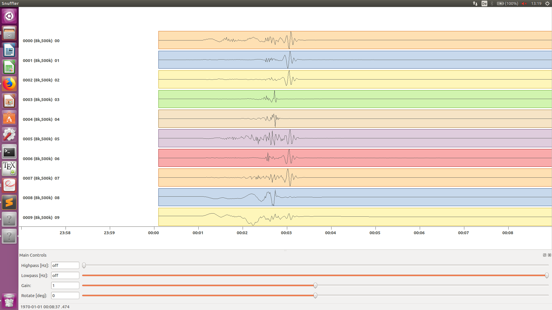
Next we can use the fomosto tool together with snuffler to inspect if the GFs look reasonable. To plot the 10 elementary GF components in a depth of 8km at a distance of 500km:
fomosto view $GF_path/AqabaMT_ak135_1.000Hz_0 --extract='8k,500k'
This looks reasonably well!
Data windowing and optimization setup
Once we are confident that the GFs are reasonable we may continue to define the optimization specific setup variables. First of all we check again the WaveformFitConfig for the waves we want to optimize. In this case we want to optimize the whole waveform from P until the end of the surface waves. As the wavetrains are very close in the very near field we do not want to have overlapping time windows, which is why we deactivate one of the WaveformFitConfigs, by setting include*=False on the `slowest` *WaveformfitConfig. So please open again $project_directory/config_geometry.yaml (if you did close the file again) and edit the respective parameter!
Also there we may define a distance range of stations taken into account, define a bandpass filter and a time window with respect to the arrival time of the respective wave. Therefore, stations that are used to optimize the P-wave do not necessarily need to be used to optimize the surface waves by defining different distance ranges. Similarly, different filters and arrival time windows maybe defined as well. These parameters are all fine for this case here!
The optimization is done in the R, T, Z rotated coordinate system to better tune, which part of the waves are optimized. That is particularly important if the S-wave is going to be used, as one would typically use only SH waves which are the S-waves in the T-component. For P-waves one would like to use the Z(vertical) component and for surface waves both components. So please make sure that in $project_directory/config_geometry.yaml under the WaveformFitConfig (name ‘any_P’) the channels list contains [Z, T] (including the brackets!)!
Finally, we fix the depth prior to 8km (upper and lower) as we only calculated GFs for that depth. $project_directory/config_geometry.yaml under the point priors:
priors:
  depth: !beat.heart.Parameter
    name: depth
    form: Uniform
    lower: [8.0]
    upper: [8.0]
    testvalue: [8.0]
Of course, in a real case this would not be fixed.
The specifications of the tapers, filters and channels that the user defined above determine which part of the data traces are used in the course of the optimization. We may inspect the raw data together with the processed data that is going to be used in the course of the optimization with
beat check FullMT --what='traces'
This should open again the snuffler window and you can interactively scroll through the traces zoom in and out, filter the traces and much more. A detailed tutorial about handling the browser is given here.
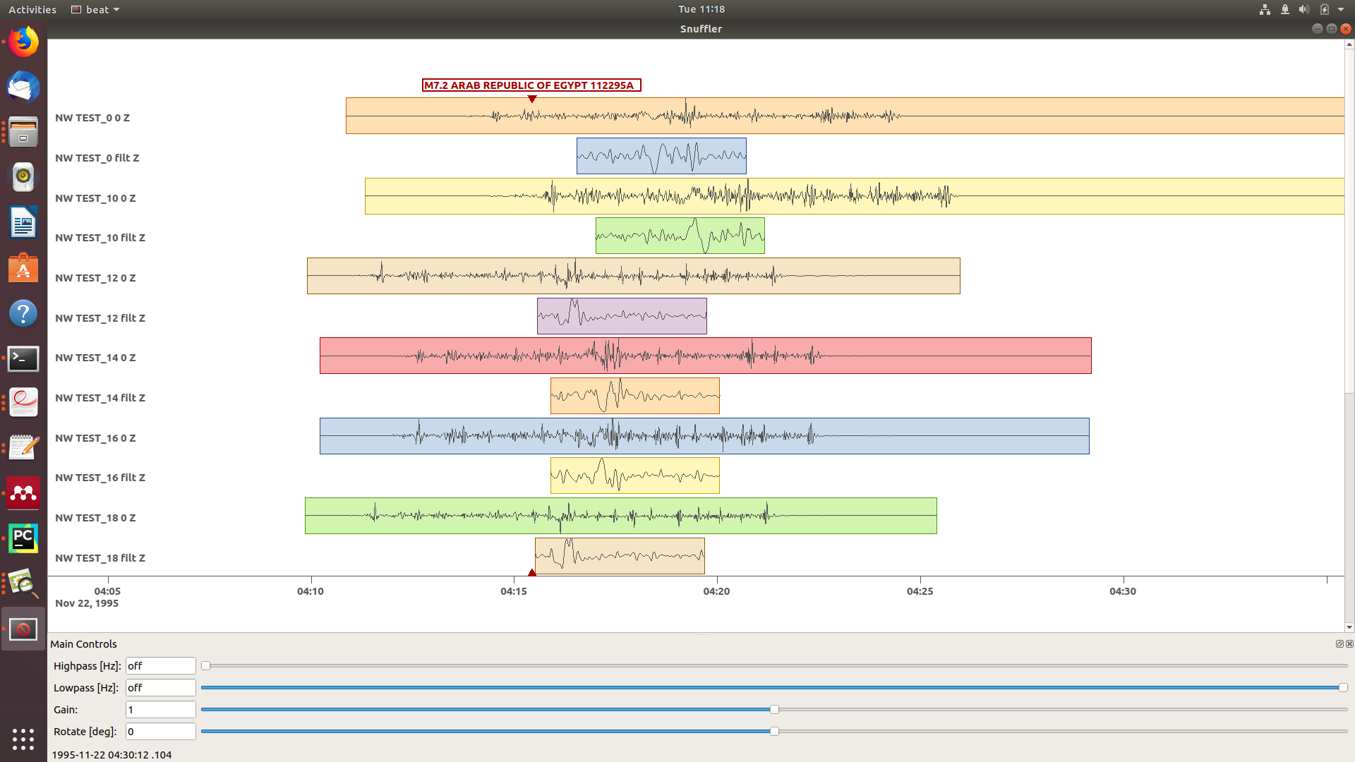
To better sort the displayed traces and to inspect the processed data we may use snufflers display options. Please right click in the window and see a menu that pops up. There, please select: Sort by Distance to sort the traces by distance to get a better picture of the setup. To see, which traces actually belong to the same station and component, please open the menu again and select Subsort by Network, Station, Channel (Grouped by Location) and Common Scale per Component. To distinguish better between the overlapping traces please select as well Color Traces and deselect Show Boxes. Your display should look something like this.
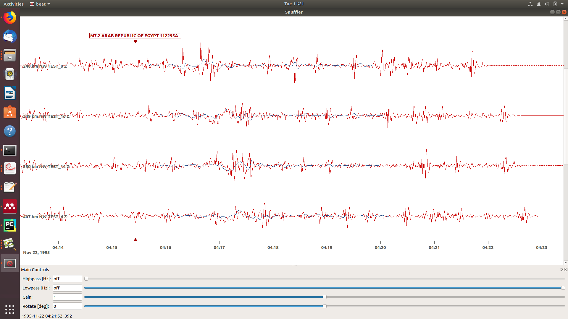
In red we see the raw data traces as stored under $project_directory/seismic_data.pkl; and in blue we see the processed data where the WaveformFitConfig parameters (see above) have been applied. The blue traces are going to be used in this form throughout the optimization. For this setup here we are good, but for future problems the user may now adjust the configuration and repeatedly check if the data windowing is satisfying. For example, the user may widen the arrival_taper times to make sure that a respective wave train is completely included in case it is cut at the taper boundary. Or in case of noisy or bad quality data a station may be completely excluded by putting its name in the blacklist parameter.
Now that we checked the optimization setup we are good to go.
Sample the solution space
Firstly, we fix the source parameters to some random value and only optimize for the noise scaling or hyperparameters (HPs). The configuration of the hyper parameter sampling, is determined by the hyper_sampler_config parameters.:
hyper_sampler_config: !beat.SamplerConfig
  name: Metropolis
  backend: csv
  progressbar: true
  buffer_size: 5000
  buffer_thinning: 1
  parameters: !beat.MetropolisConfig
    tune_interval: 50
    proposal_dist: Normal
    check_bnd: true
    rm_flag: false
    n_jobs: 1
    n_steps: 25000
    n_chains: 20
    thin: 5
    burn: 0.5
Here we use an adaptive Metropolis algorithm to sample the solution space. How many different random source parameters are chosen and how often the sampling is repeated is controlled by n_chains (default:20). In case there are several CPUs available the n_jobs parameter determines how many processes (Markov Chains (MCs)) are sampled in parallel. Each MC will contain 25k samples (n_steps) and every 50 samples the step-size will be adjusted (tune_interval). You may want to increase that now! To start the sampling please run
beat sample FullMT --hypers
This reduces the initial search space from 40 orders of magnitude to usually 5 to 10 orders. Checking the $project_directory/config_geometry.yaml, the HPs parameter bounds show something like:
hyperparameters:
  h_any_P_0_Z: !beat.heart.Parameter
    name: h_any_P_0_Z
    form: Uniform
    lower: [-3.0]
    upper: [3.0]
    testvalue: [0.0]
  h_any_P_1_T: !beat.heart.Parameter
    name: h_any_P_1_T
    form: Uniform
    lower: [-3.0]
    upper: [2.0]
    testvalue: [-0.5]
Now that we have an initial guess on the hyperparameters we can run the optimization using the default sampling algorithm, a Sequential Monte Carlo sampler. The sampler can effectively exploit the parallel architecture of nowadays computers. The n_jobs number should be set to as many CPUs as possible in the configuration file.:
sampler_config: !beat.SamplerConfig
  name: SMC
  backend: bin
  progressbar: true
  buffer_size: 1000
  buffer_thinning: 50
  parameters: !beat.SMCConfig
    n_chains: 500
    n_steps: 100
    n_jobs: 4
    tune_interval: 10
    coef_variation: 1.0
    stage: 0
    proposal_dist: MultivariateNormal
    check_bnd: true
    update_covariances: false
    rm_flag: true
Note
n_chains divided by n_jobs MUST yield a whole number! An error is going to be thrown if this is not the case!
Here we use 4 cpus (n_jobs) - you can change this according to your systems specifications. Finally, we sample the solution space with:
beat sample FullMT
Note
The reader might have noticed the two different backends that have been specified in the SamplerConfigs, “csv” and “bin”. Here we refer to the backend section that describe these further.
Note
For more detailed search of the solution space please modify the parameters ‘n_steps’ and ‘n_chains’ for the SMC sampler in the $project_directory/config_geometry.yaml file to higher numbers. Depending on these specifications and the available hardware the sampling may take several hours/few days. Further remarks regarding the configuration of the sampler can be found here .
Summarize the results
The sampled chain results of the PT sampler are stored in separate files and have to be summarized.
Note
Only for MomentTensor MTSource: The moment tensor components have to be normalized again with respect to the magnitude.
To summarize all the stages of the sampler please run the summarize command.:
beat summarize FullMT
If the final stage is included in the stages to be summarized also a summary file with the posterior quantiles will be created. If you check the summary.txt file (path then also printed to the screen):
vi $project_directory/geometry/summary.txt
For example for the first 4 entries (mee, med, posterior like-lihood, north-shift), the posterior pdf quantiles show:
                         mean        sd  mc_error       hpd_2.5      hpd_97.5
mee__0             -0.756400  0.001749  0.000087     -0.759660     -0.752939
med__0             -0.256697  0.000531  0.000024     -0.257759     -0.255713
like__0         89855.787301  2.742033  0.155631  89849.756559  89859.893765
north_shift__0     19.989398  0.010010  0.000496     19.970455     20.008629
As this is a synthetic case with only little noise it is not particularly surprising to get such steeply peaked distributions.
Plotting
Now to the point that you all have been waiting for ;) the result in pictures. To see the waveform fit of the posterior maximum likelihood solution. In the $beat_models run:
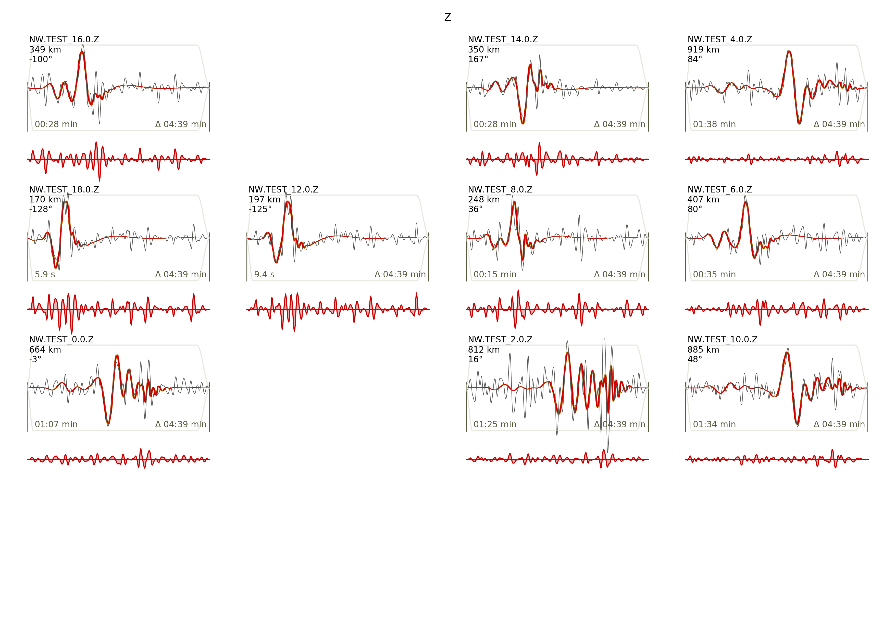
beat plot FullMT waveform_fits --nensemble=100
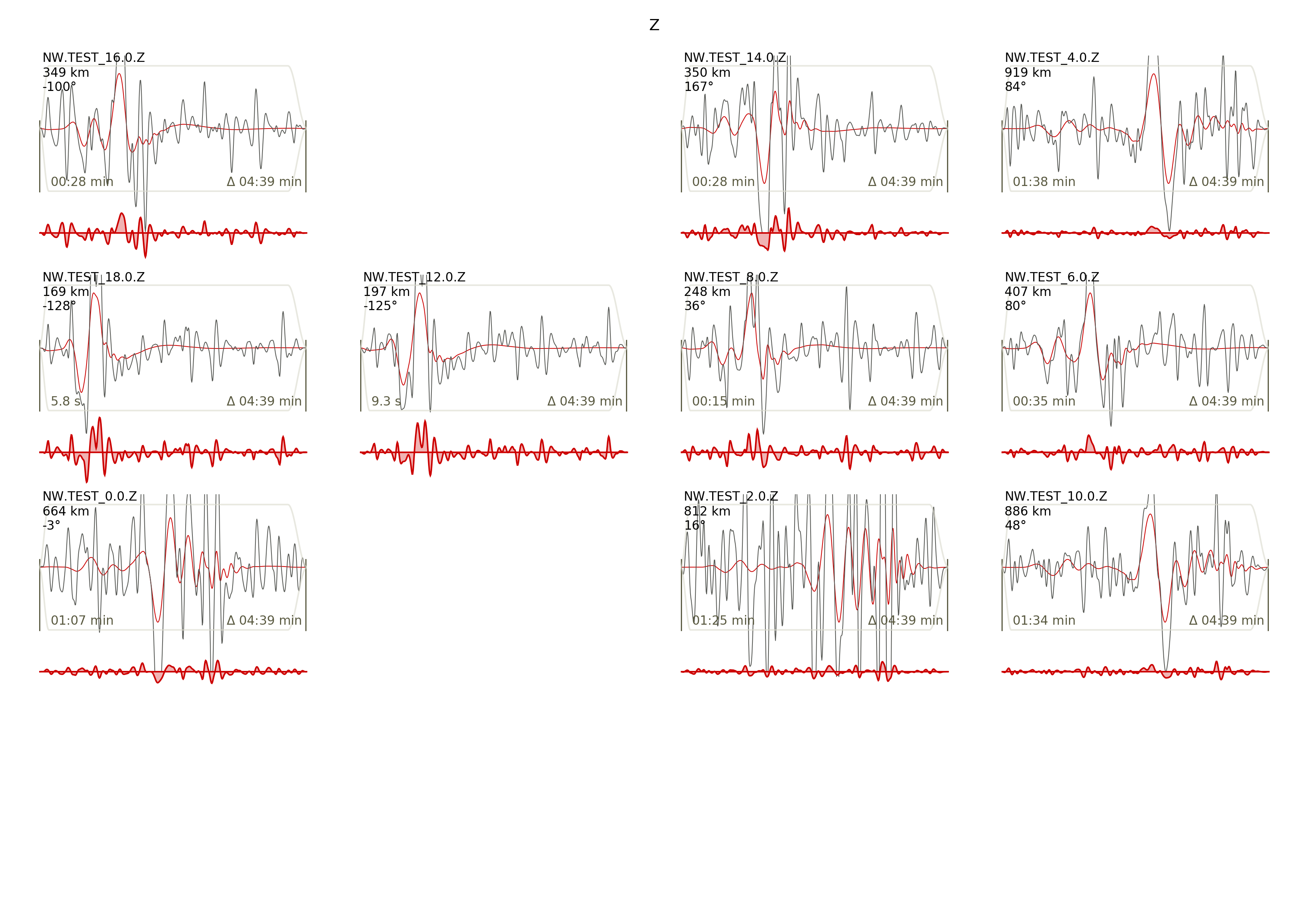
If it worked it will produce a pdf with several pages output for all the components for each station that have been used in the optimization. The black waveforms are the unfiltered data. Red are the best fitting synthetic traces. Light grey and light red are the filtered, untapered data and synthetic traces respectively. The red data trace below are the residual traces between data and synthetics. The Z-components from our stations should look something like this. The nensemble parameter defines the number of draws that are taken from the posterior probability density to forward calculate an ensemble of synthetic waveforms.
The waveform fits for a specific point in the solution space may be produced by setting the testvalues in the Prior distributions of the config file. Here, these values got already set to the true solution. So we can compare if our best estimated source parameters are reasonable compared to the true ones.
beat plot FullMT waveform_fits --reference
Again looking at the Z-components of the traces shows that our estimate is far off to the true test value.
The following command produces a ‘.png’ file with the final posterior distribution. In the $beat_models run:
beat plot FullMT stage_posteriors --reference --stage_number=-1 --format='png'
It may look like this.
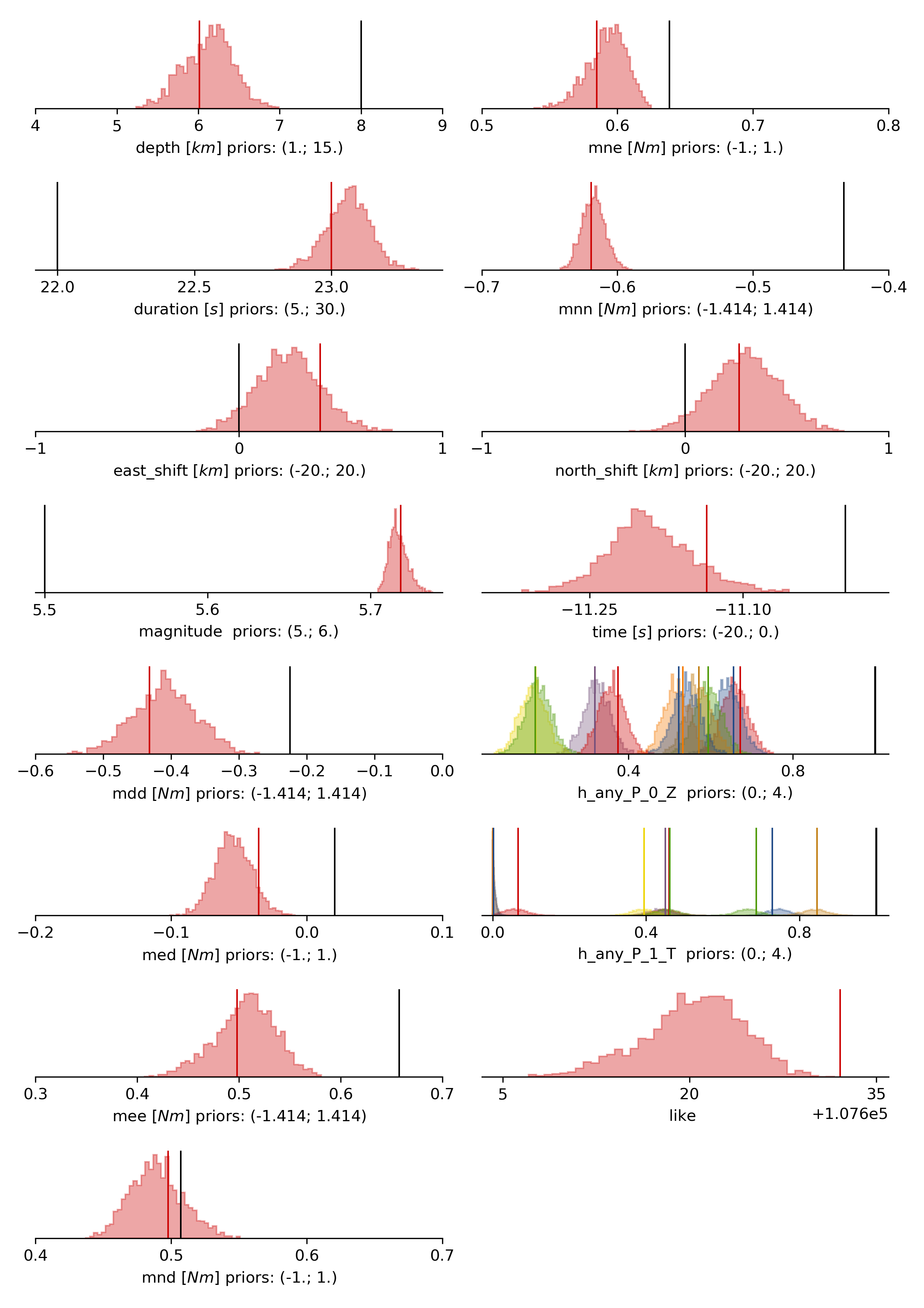
The vertical black lines are the true values and the vertical red lines are the maximum likelihood values. We see that the true solution is not comprised within the marginals of all parameters. This may have several reasons. In the next section we will discuss and investigate the influence of the noise characteristics.
To get an image of parameter correlations (including the true reference value in red) of moment tensor components, the location and the magnitude. In the $beat_models run:
beat plot FullMT correlation_hist --reference --stage_number=-1 --format='png' --varnames='mee, med, mdd, mnn, mnd, mne, north_shift, east_shift, magnitude'
This will show an image like that.
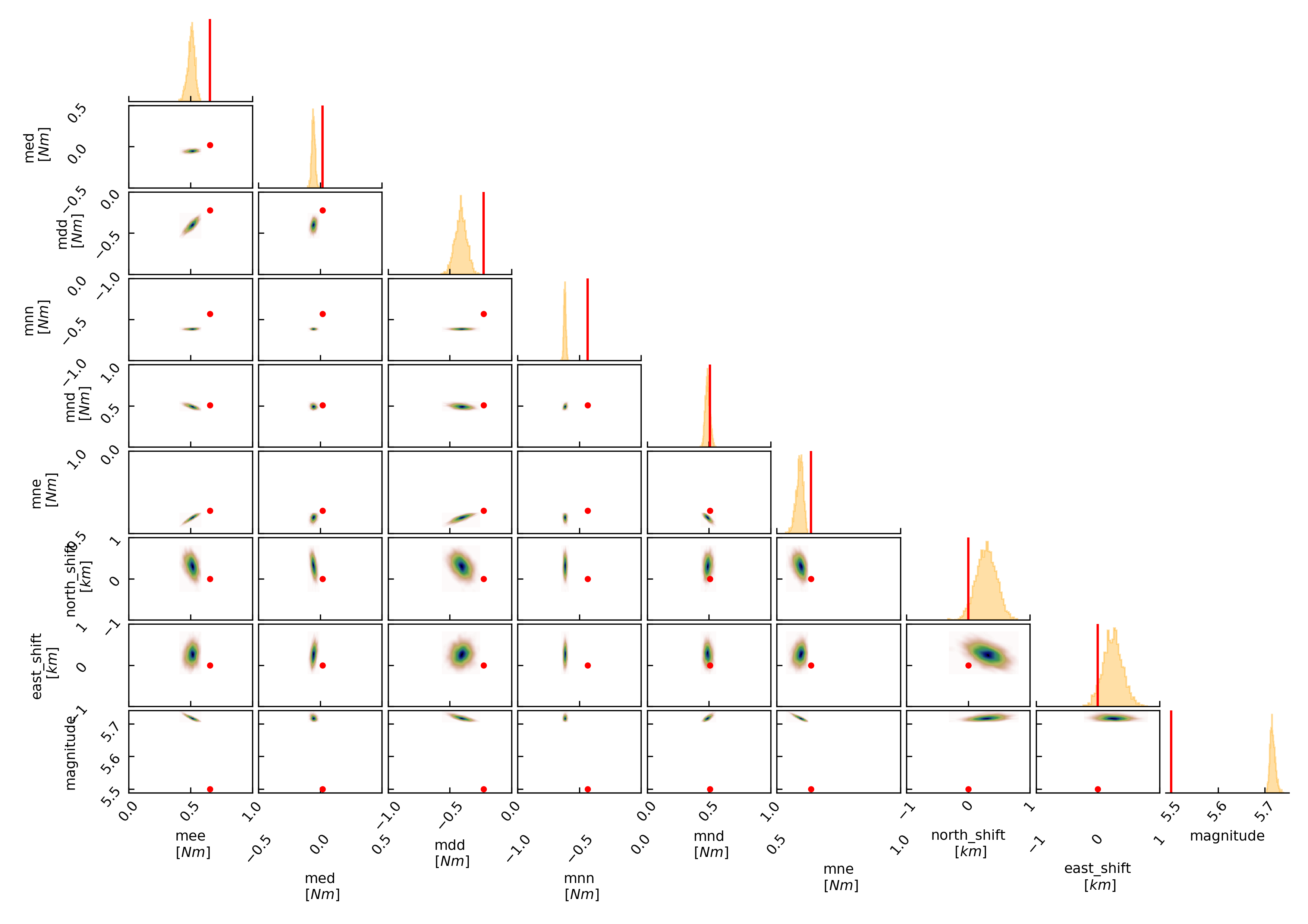
This shows 2d kernel density estimates (kde) and histograms of the specified model parameters. The darker the 2d kde the higher the probability of the model parameter. The red dot and the vertical red lines show the true values of the target source in the kde plots and histograms, respectively.
The varnames option may take any parameter that has been optimized for. For example one might also want to try –varnames=’duration, time, magnitude, north_shift, east_shift’. If it is not specified all sampled parameters are taken into account.
Seismic noise estimation
If we have poor knowledge of the noise in the data, the model parameter estimates may be poor and the true parameters are not covered by the distributions (as was the case above). In the previous run we used a data covariance matrix of the form of an identity matrix with only the noise variance in the diagonal. Under the seismic_config you find the configuration for the noise analyser, which looks like that:
noise_estimator: !beat.SeismicNoiseAnalyserConfig
  structure: variance
  pre_arrival_time: 3.0
The structure argument refers to the structure of the covariance matrix that is estimated on the data, prior to the synthetic P-wave arrival. The argument pre_arrival_time refers to the time before the P-wave arrival. 3.0 means that the noise is estimated on each data trace up to 3. seconds before the synthetic P-wave arrival. Obviously, in the previous run the white-noise assumption was not working well. So we may set the structure to exponential to also estimate noise covariances depending on the shortest wavelength in the data, following [Duputel2012].
Other options are to import to use the covariance matrices that have been imported with the data Also the option non-toeplitz to estimate non-stationary, correlated noise on the residuals following [Dettmer2007].
Clone setup into new project
Now we want to repeat the sampling with the noise structure set to non-toeplitz, but we want to keep the previous results as well as the configuration files unchanged for keeping track of our work. So we can use again the clone function to clone the current setup into a new directory.:
beat clone FullMT FullMT_nont --copy_data --datatypes=seismic
Now we can change the noise_estimator to use non-toeplitz structured covariance matrices in the new project directory FullMT_nont keeping all the other configurations identical.:
noise_estimator: !beat.SeismicNoiseAnalyserConfig
  structure: non-toeplitz
  pre_arrival_time: 3.0
In this case the values from the priors and hypers testvalues are used as reference to calculate the initial residuals, which are being used to estimate the covariance matrices. This may produce heavily biased results in case these values are far off the true source parameters. Therefore, we have to update the non-Toeplitz covariance estimates in the course of the samping! We can do this by setting the update_covariances parameter in the SMC parameters to true.:
sampler_config: !beat.SamplerConfig
  name: SMC
  progressbar: true
  buffer_size: 5000
  buffer_thinning: 10
  parameters: !beat.SMCConfig
    n_chains: 500
    n_steps: 100
    n_jobs: 4
    tune_interval: 10
    coef_variation: 1.0
    stage: 0
    proposal_dist: MultivariateNormal
    check_bnd: true
    update_covariances: true    % <-- HERE! ;)
    rm_flag: true
Please go ahead and repeat the run with the steps from above using this configuration!
Again plotting the parameter marginals with:
beat plot FullMT_nont stage_posteriors --reference --stage_number=-1 --format='png'
This will show an image like that.
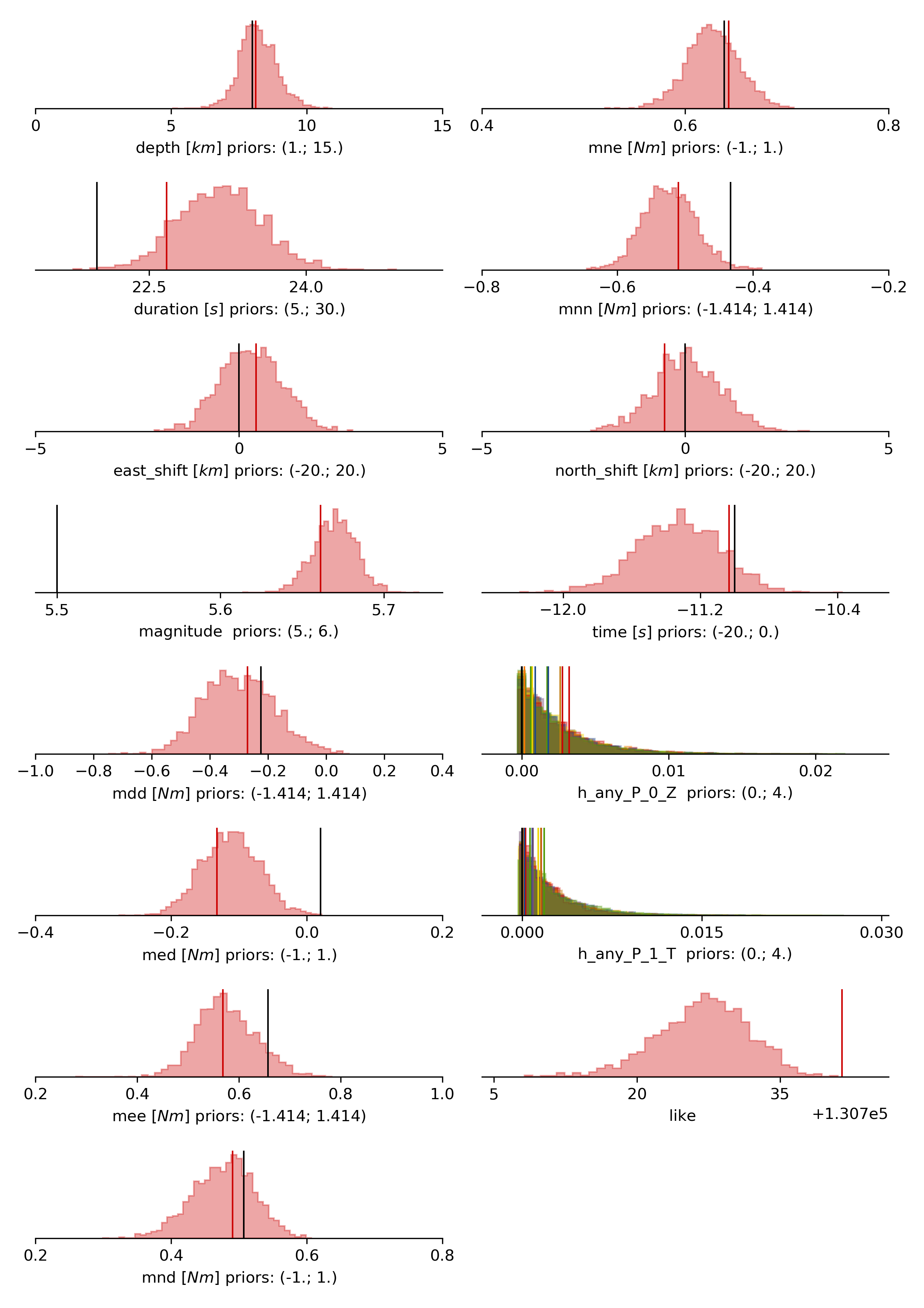
Now we are doing much better regarding the moment tensor components. However, the magnitude is still overestimated, but there is not much we can do about that so far with such data.
Please also go ahead and check out the other plots like the hudson or fuzzy_beachball.
References
Dettmer, Jan and Dosso, Stan E. and Holland, Charles W., Uncertainty estimation in seismo-acoustic reflection travel time inversion, The Journal of the Acoustical Society of America, DOI:10.1121/1.2736514
Duputel, Zacharie and Rivera, Luis and Fukahata, Yukitoshi and Kanamori, Hiroo, Uncertainty estimations for seismic source inversions, Geophysical Journal International, DOI:10.1111/j.1365-246X.2012.05554.x