Example 4a: Static finite-fault estimation, uniform patch discretization

In this example we will determine a variable slip distribution for the L’aquila 2009 earthquake by using static InSAR data. We will use uniform discretization of fault patches across the fault surface. The data is the exact same from Example 3, where the overall geometry of the fault plane was estimated. It is a requirement to have Example 3 completed in order to follow the instructions and commands given in this example.

Please make sure that you are one level above the Laquila project folder (created earlier).:

cd $beat_models_path

Init

In this example you will first make use of the mode argument. The default is: geometry, which is why it was not necessary to specify it in the earlier examples. Now we will always have to set mode to ffi, which is an abbreviation for finite-fault-inference. The following command will create a configuration file for the ffi mode called config_ffi.yaml right next to the config_geometry.yaml:

beat init Laquila --mode='ffi' --datatypes=geodetic

It will load the config_geometry.yaml and port arguments that have been specified before to ensure consistency and will only use geodetic data.

The main differences in the two configuration files are in the geodetic_config.gf_config and the problem_config. You may want to have a first glance at the new config. The general structure is the same and the argument names are chosen to give the user an initial idea what these are for. A short explanation for each argument is again given in the module API here, where you can use the search function of your browser to find the argument of interest.

Calculate Greens Functions

For the distributed slip optimization a reference fault has to be defined that determines the overall geometry. Once this has been done the problem becomes linear as the only unknown parameters are the slips in rake perpendicular and rake parallel direction. The fault geometry needs to be defined in the geodetic.gf_config.reference_sources.:

gf_config: !beat.GeodeticLinearGFConfig
  store_superdir: /home/vasyurhm/GF/Laquila
  reference_model_idx: 0
  n_variations: [0, 1]
  earth_model_name: ak135-f-average.m
  nworkers: 4
  reference_sources:
  - !beat.sources.RectangularSource
    lat: 42.29
    lon: 13.35
    north_shift: 5542.073672733207
    east_shift: 10698.176839272524
    elevation: 0.0
    depth: 2926.702988951863
    time: 2009-04-06 01:32:49.19
    stf: !pf.HalfSinusoidSTF
      duration: 0.0
      anchor: 0.0
    stf_mode: post
    strike: 144.48588106798306
    dip: 54.804317242125464
    rake: -114.58259929068664
    length: 12219.56636799338
    width: 9347.802691161543
    velocity: 3500.0
    slip: 0.5756726498300268
  discretization: uniform
  discretization_config: !beat.UniformDiscretizationConfig
    extension_widths:
    - 0.6
    extension_lengths:
    - 0.4
    patch_widths:
    - 2.0
    patch_lengths:
    - 2.0
  sample_rate: 1.1574074074074073e-05

The values shown above are parts of the MAP solution from the optimization from Example 3 . The results can been imported through the import command specifying the –results option. We want to import the results from the Laquila project_directory from an optimization in geometry mode and we want to update the geodetic part of the config_ffi.yaml:

beat import Laquila --results=Laquila --mode='ffi' --datatypes=geodetic --import_from_mode=geometry

Of course, these values could be edited manually to whatever the user deems reasonable.

Warning

The reference point(s) on the reference_fault(s) are the top, central point of the fault(s)! Ergo the depth parameter(s) relate(s) to the top edge(s) of the fault(s).

Under the discretization attribute we can select the way of discretizing the fault surface into patches, now the default uniform is set. This attribute determines the discretization_config below. Here, we need to specify the dimensions of the patches we want to discretize the reference fault(s) into. The patch_widths and patch_lengths arguments have to be lists and the respective entry needs to result in square patches. The parameters extension_withs and extension_lengths specify by how much the reference fault(s) should be extended in each direction. Example: 0.1 means that the fault is extended by 10% of its width/length value in each direction and 0. means no extension.

Once we decided for the discretization and the reference fault values we can create the discretized fault through.:

beat build_gfs Laquila --datatypes=geodetic --mode=ffi

This will create a directory ($linear_gfs): Laquila/ffi/linear_gfs where the fault geometry is saved as a pickle file ‘fault_geometry.pkl’. We can inspect the geometry of the resulting extended discretized fault wrt. the reference fault with:

beat check Laquila --what=discretization --mode=ffi

This will open an interactive 3d plot of the fault geometry, which looks along the lines of

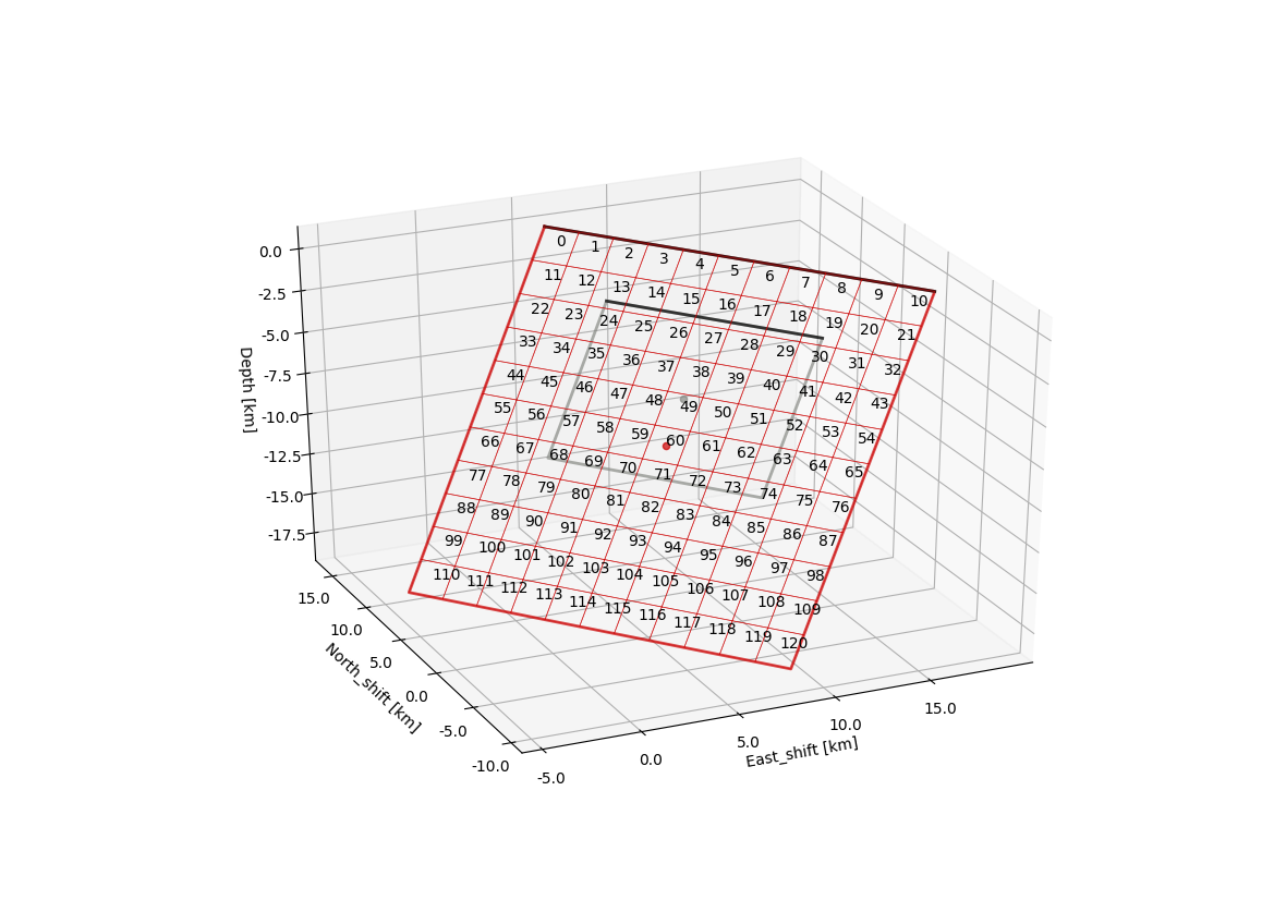
The grey rectangle shows the geometry of the fault specified under reference_sources and the red rectangle(s) show the extended fault with the respective discretization of the sub-patches. The grey and red dots mark the centres of the reference_fault(s) and the extended faults, respectively. The numbers are the indexes of the repsective sub-patch in the Green’s Function matrix we are going to calculate next.

Note

If the upper edge of the fault would intersect the surface (no topography assumed) due to the extension it is truncated at the intersection and not extended further. Which is why the extent of the red fault is asymmetric around the grey reference fault in dip-direction.

To repeat the fault discretization after changing some parameters please add the –force option and the previously fault geometry will be overwritten.:

beat build_gfs Laquila --datatypes=geodetic --mode=ffi --force

The next command starts the calculation of the linear Green’s Function matrixes (also called library) using nworkers CPUs in parallel with unit slip in each slip-direction.:

beat build_gfs Laquila --datatypes=geodetic --mode=ffi --execute

Note

The slip components are not dip-slip and strike-slip, but rake-parallel (uparr in config_ffi.yaml priors) and rake-perpendicular (uperp in config_ffi.yaml priors) wrt to reference_fault(s) rake angle(s). This is following the convention of [Minson2013]. In addition to that there is the component utens, which is normal to the previously mentioned components and would be needed to simulate tensile opening or closing. We ignore that here as we want to model a shear-dislocation.

This will create two files for each GF library in the $linear_gfs directory:

• geodetic_uparr_static_0.traces.npy a numpy array containing the linear GFs

• geodetic_uparr_static_0.yaml a yaml file with the meta information

Now we are ready to prepare the optimization setup.

Optimization setup

Under the problem_config we find the parameters that we need to adjust:

problem_config: !beat.ProblemConfig
  mode: ffi
  mode_config: !beat.FFIConfig
    regularization: none
    npatches: 121
    initialization: random
  source_types: [RectangularSource]
  stf_type: HalfSinusoid
  decimation_factors:
    geodetic: 1
    seismic: 1
  n_sources: [1]
  datatypes: [geodetic, seismic]
  hyperparameters:
    h_SAR: !beat.heart.Parameter
      name: h_SAR
      form: Uniform
      lower: [-20.0]
      upper: [20.0]
      testvalue: [0.0]
  priors:
    uparr: !beat.heart.Parameter
      name: uparr
      form: Uniform
      lower: [-0.05]
      upper: [6.0]
      testvalue: [1.15]
    uperp: !beat.heart.Parameter
      name: uperp
      form: Uniform
      lower: [-0.3]
      upper: [4.0]
      testvalue: [0.5]
    utens: !beat.heart.Parameter
      name: utens
      form: Uniform
      lower: [0.0]
      upper: [0.0]
      testvalue: [0.0]
  hierarchicals:
    Laquila_ascxn_azimuth_ramp: !beat.heart.Parameter
      name: Laquila_ascxn_azimuth_ramp
      form: Uniform
      lower:
      - -0.00043773457168120667
      upper:
      - -0.00043773457168120667
      testvalue:
      - -0.00043773457168120667
    Laquila_ascxn_offset: !beat.heart.Parameter
      name: Laquila_ascxn_offset
      form: Uniform
      lower:
      - -0.004496268249748271
      upper:
      - -0.004496268249748271
      testvalue:
      - -0.004496268249748271
    Laquila_ascxn_range_ramp: !beat.heart.Parameter
      name: Laquila_ascxn_range_ramp
      form: Uniform
      lower:
      - -0.00023808150002277328
      upper:
      - -0.00023808150002277328
      testvalue:
      - -0.00023808150002277328
    Laquila_dscxn_azimuth_ramp: !beat.heart.Parameter
      name: Laquila_dscxn_azimuth_ramp
      form: Uniform
      lower:
      - 4.978325480108451e-05
      upper:
      - 4.978325480108451e-05
      testvalue:
      - 4.978325480108451e-05
    Laquila_dscxn_offset: !beat.heart.Parameter
      name: Laquila_dscxn_offset
      form: Uniform
      lower:
      - -0.003754963750062188
      upper:
      - -0.003754963750062188
      testvalue:
      - -0.003754963750062188
    Laquila_dscxn_range_ramp: !beat.heart.Parameter
      name: Laquila_dscxn_range_ramp
      form: Uniform
      lower:
      - -0.00025072248953317104
      upper:
      - -0.00025072248953317104
      testvalue:
      - -0.00025072248953317104

Note

The npatches parameter should not be manually adjusted. It is automatically set by running the fault discretizeation step during GF calculation(above).

Hierarchicals

Please notice the hierarchicals parameters! These are the MAP parameters for the orbital ramps for each radar scene that have been optimized in Example 3 . These parameters are imported if the ramp correction under corrections in the geodetic_config was set to True.:

corrections_config: !beat.GeodeticCorrectionsConfig
  euler_poles:
  - !beat.EulerPoleConfig
    enabled: false
  ramp: !beat.RampConfig
    dataset_names:
    - Laquila_dscxn
    - Laquila_ascxn
    enabled: true
  strain_rates:
  - !beat.StrainRateConfig
    enabled: false

The default is to fix these ramp parameters during the static distributed slip optimization, because leaving them open often results in tradeoffs with patches at greater depth and thus artificial slip is optimized at greater depth. Nevertheless, the user may want to try out to free the upper and lower bounds again to include the parameters into the optimization.

..note:: The EulerPole and StrainRate corrections are useful for interseismic studies and will be covered in another tutorial.

Priors

The upper and lower bounds of the two prior variables can be adjusted to reduce the solution space (slip parameters [m]). For the L’aquila earthquake it is highly unlikely to have 6 meters of slip, which is simply the default parameter. A maximum slip of 2 meters in slip parallel direction may be more reasonable. In order to be able to sample the zero value at the lower bound it is necessary to allow for some backslip- ergo negative uparr; here 0.1 might be a reasonable choice.

To also allow for variable rake angles across the fault we may want to allow some rake perpendicular slip. Here the lower and upper bounds should be set to -1. and 1., respectively.

Note

In order to fix a variable at a certain value, the lower and upper bounds as well as the testvlue need to be set to the same value.

Regularization

The regularization argument should be set to laplacian to introduce a smoothing constraint that penalizes high slip gradients between neighboring patches. Once this is enabled we need to update the configuration file to initialize the slip-smoothing weight as a random variable in the optimization [Fukuda2008]. Adding the –diff option will display the changes to the config to screen instead of applying them to the file.:

beat update Laquila --mode=ffi --diff --parameters=hypers

Once happy with the displayed changes the changes will be applied to the file with:

beat update Laquila --mode=ffi --parameters=hypers

Note

The None regularization would be used if covariance matrices that describe the theory errors for the velocity model and/or the fault geometry have been estimated [Duputel2014] , [Ragon2018]. How to do that in BEAT will be part of another tutorial in the future.

Sample the solution space

Please refer to the ‘Sample the solution space section’ of example 3 example for a more detailed description of the sampling and associated parameters.

Firstly, we only optimize for the noise scaling or hyperparameters (HPs) including the laplacian smoothing weight:

beat sample Laquila --hypers --mode=ffi

Checking the $project_directory/config_ffi.yaml, the hyperparameter bounds show something like:

hyperparameters:
h_SAR: !beat.heart.Parameter
  name: h_SAR
  form: Uniform
  lower: [-1.0]
  upper: [5.0]
  testvalue: [2.0]
h_laplacian: !beat.heart.Parameter
  name: h_laplacian
  form: Uniform
  lower: [-5.0]
  upper: [5.0]
  testvalue: [0.5]

Markov Chain initialization

The initialization argument determines at which point in the solution space to initialize the Markov Chains. The default value random simply draws a random point in the solution space from the prior distributions for each Markov Chain to be sampled. However, as we are using a laplacian smoothing constraint we can use the non-negative least-squares solution as a starting value for a randomly drawn smoothing weight (from the initial guess on the h_laplacian parameter range) [Fukuda2008]. To do, so we need to set the initialization to “lsq”:

mode_config: !beat.FFIConfig
  regularization: laplacian
  npatches: 121
  initialization: lsq

The ‘n_jobs’ number should be set to as many CPUs as the user can spare under the sampler_config. The number of sampled MarkovChains and the number of steps for each chain of the SMC sampler should be set to high values as we are optimizing now for ca 250 random variables (if the values from the tutorial haven’t been altered by the user); for example to 5000 and 400, respectively.

Warning

With these sampler parameters a huge amount of samples are going to be stored to disk! With the values from the tutorial approximately 140GB of samples are created in the course of the sampling. Please see example 0 for an instruction on how to keep only the important samples to reduce the disk usage. Another way to reduce the required disc space is through the buffer_thinning parameter described here.

Finally, we are set to run the full optimization for the static slip-distribution with:

beat sample Laquila --mode=ffi

Summarize and plotting

After the sampling successfully finished, the final stage results have to be summarized with:

beat summarize Laquila --stage_number=-1 --mode=ffi

After that several figures illustrating the results can be created.

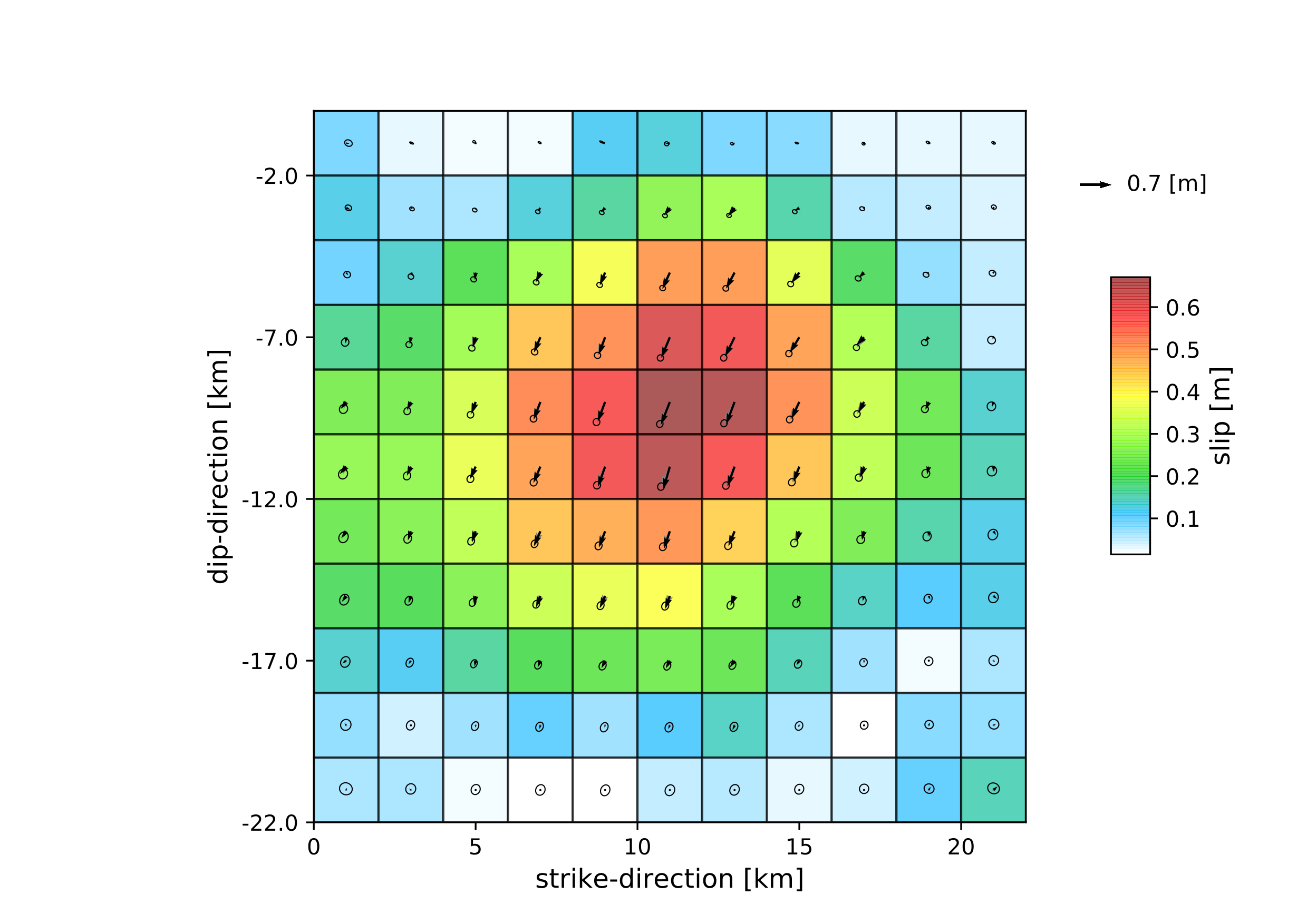
For the slip-distribution please run:

beat plot Laquila slip_distribution --mode=ffi

To get histograms for the laplacian smoothing, the noise scalings and the posterior likelihood please run:

beat plot Laquila stage_posteriors --stage_number=-1 --mode=ffi --varnames=h_laplacian,h_SAR,like

For a comparison between data, synthetic displacements and residuals for the two InSAR tracks in a local coordinate system please run:

beat plot Laquila scene_fits --mode=ffi

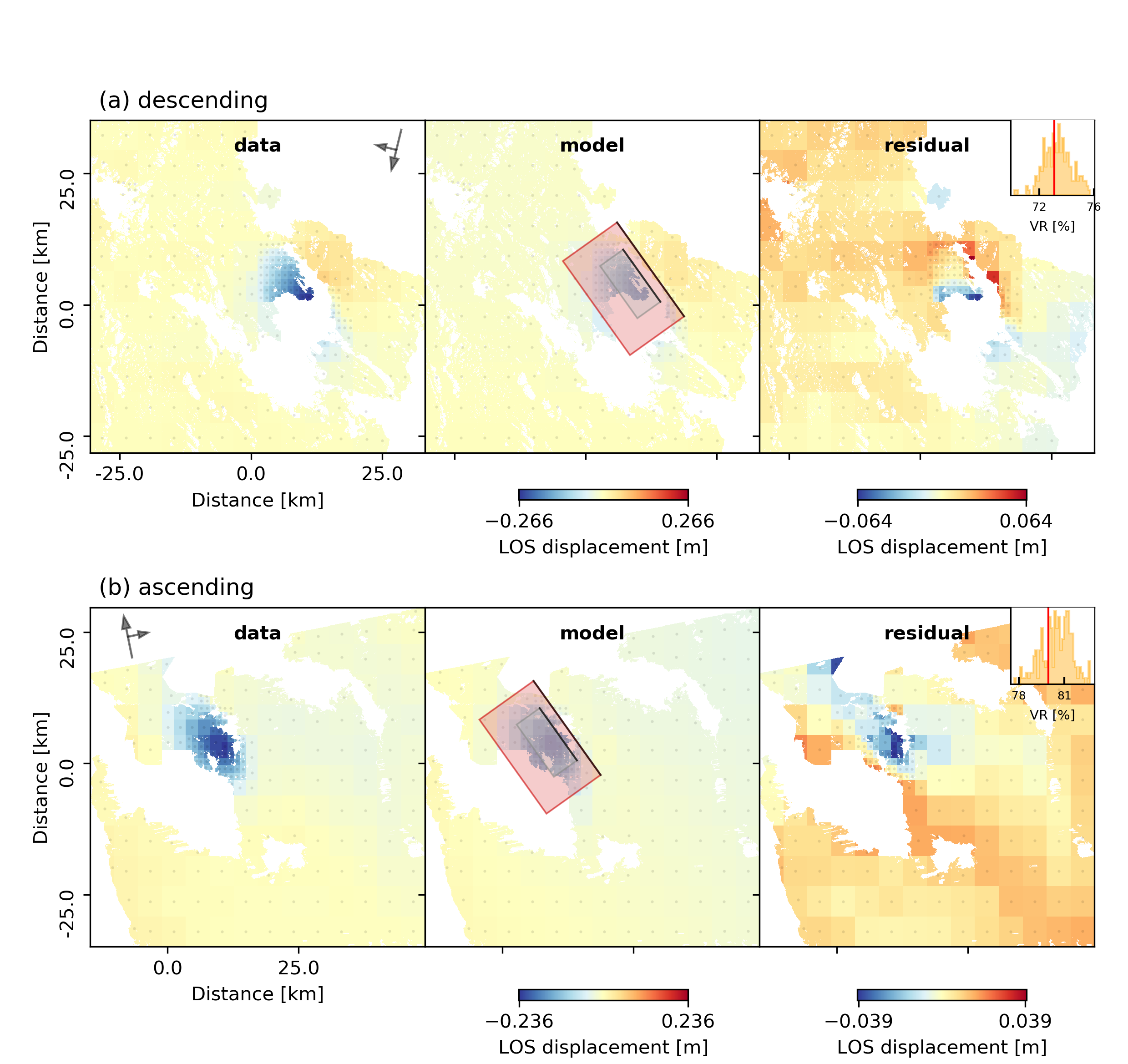
The plot should show something like this. Here the residuals are displayed with an individual color scale according to their minimum and maximum values.

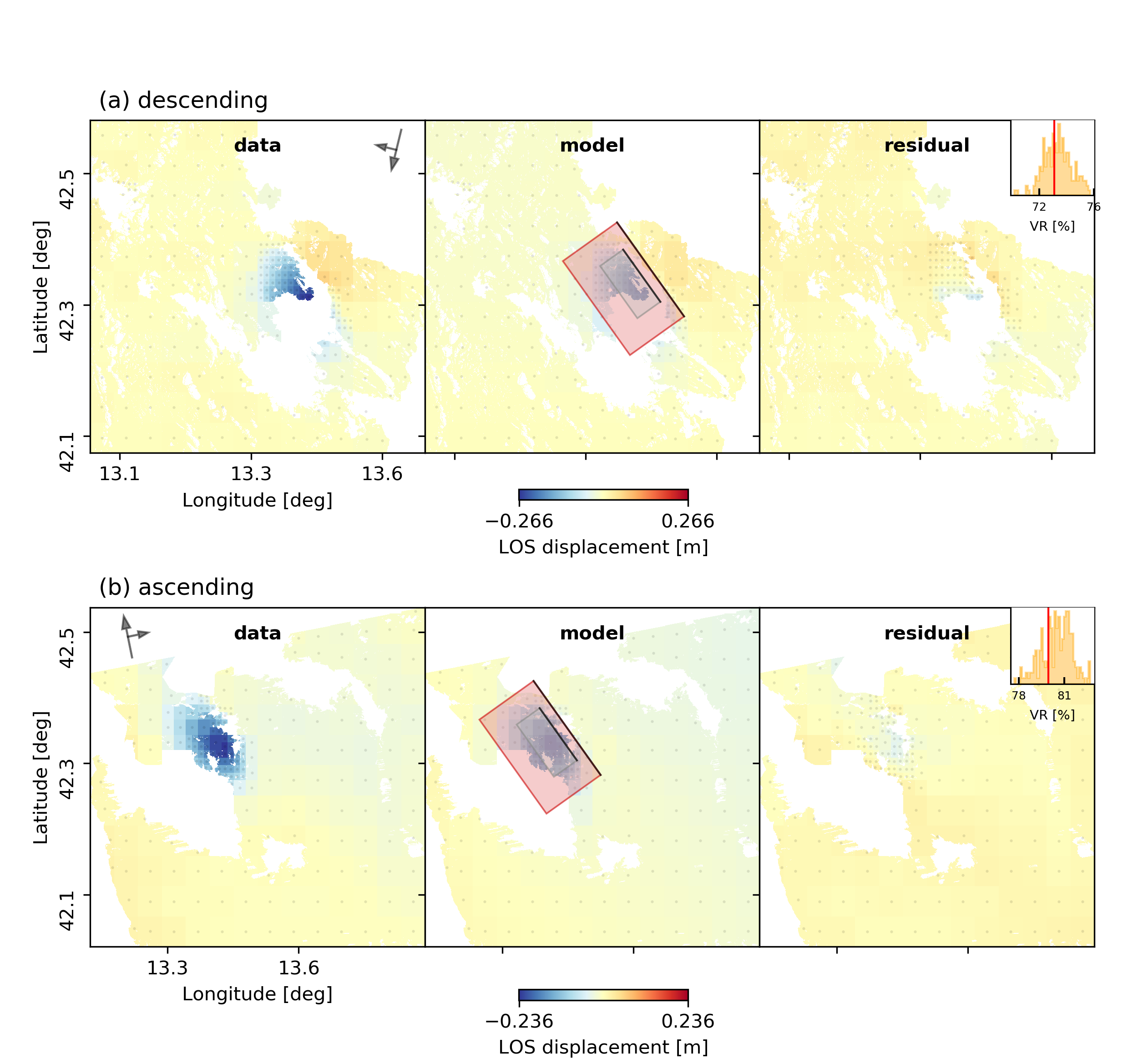
For a plot using the global geographic coordinate system where the residuals have the same color bar as data and synthetics please run:

beat plot Laquila scene_fits --mode=ffi --plot_projection=latlon

References

[Duputel2014]

Duputel, Z., Agram, P. S., Simons, M., Minson, S. E., and Beck, J. L. (2014). Accounting for prediction uncertainty when inferring subsurface fault slip. Geophysical Journal International, 197(1):464–482

[Fukuda2008] (1,2)

Fukuda, J. and Johnson, K. M. (2008). A fully Bayesian inversion for spatial distribution of fault slip with objective smoothing. Bulletin of the Seismological Society of America, 98(3):1128–1146

[Ragon2018]

Ragon, T., Sladen, A., Simons, M. Accounting for uncertain fault geometry in earthquake source inversions – I: theory and simplified application, Geophysical Journal International, 214(2):1174–1190