Example 7: Static tensile finite-fault inference, resolution based patch discretization
In this example we will determine a variable opening distribution for the magmatic intrusion at Fernandina during the time Dec 2014 - June 2018. This example The data is the exact same from Example 6, where the overall geometry of the dike was estimated. Here we use resolution based discretization of dividing the dike surface into smaller patches following the approach of [Atzori2011]. It is assumed that the reader has Example 6 completed before following this example.
Init
In this example you will make use of the mode argument. The default is: geometry, which is why it was not necessary to specify it in the earlier example 6. Now we will always have to set mode to ffi, which is an abbreviation for finite-fault-inference. The following command will create a configuration file for the ffi mode called config_ffi.yaml right next to the config_geometry.yaml:
beat init Fernandina --mode='ffi' --datatypes=geodetic
It will load the config_geometry.yaml and port arguments that have been specified before to ensure consistency and will only use geodetic data.
The main differences in the two configuration files are in the geodetic_config.gf_config and the problem_config. You may want to have a first glance at the new config. The general structure is the same and the argument names are chosen to give the user an initial idea what these are for. A short explanation for each argument is again given in the module API here, where you can use the search function of your browser to find the argument of interest.
Optimization setup
To infer a tensile slip component instead of a shear slip component in BEAT, priors parameters need to be adjusted. Users that are familiar with the variable shear slip inference on a fault will not find many differences compared to such a scenario. Under priors the problem_config we find the default parameters that we need to adjust. The default is estimation of slip in rake parallel uparr and rake perpendicular uperp direction and no tensile utens slip.:
priors:
  uparr: !beat.heart.Parameter
    name: uparr
    form: Uniform
    lower: [-0.05]
    upper: [6.0]
    testvalue: [1.15]
  uperp: !beat.heart.Parameter
    name: uperp
    form: Uniform
    lower: [-0.3]
    upper: [4.0]
    testvalue: [0.5]
  utens: !beat.heart.Parameter
    name: utens
    form: Uniform
    lower: [0.0]
    upper: [0.0]
    testvalue: [0.0]
This needs to be adjusted to sth like the following to enable the tensile slip and disable the shear slip components. (If we remember from earlier tutorials, a variable can be fixed by setting, upper, lower and testvalue fields to the same value, in our case zero):
priors:
  uparr: !beat.heart.Parameter
    name: uparr
    form: Uniform
    lower:
    - 0.0
    upper:
    - 0.0
    testvalue:
    - 0.0
  uperp: !beat.heart.Parameter
    name: uperp
    form: Uniform
    lower:
    - 0.0
    upper:
    - 0.0
    testvalue:
    - 0.0
  utens: !beat.heart.Parameter
    name: utens
    form: Uniform
    lower:
    - 0.0
    upper:
    - 3.0
    testvalue:
    - 0.4
Note
Mixed setups of tensile and shear-slip components is possible as well. The priors to each component need to be set accordingly, such that there is no zero fixed component.
Warning
The slip prior components need to be correctly configured prior to dike discretization, as these tell the discretization algorithm which slip components are present in the model setup! They have big impact on the outcome!!!
Calculate Greens Functions
For the distributed opening estimation a reference dike has to be defined that determines the overall geometry. Once this has been done the problem becomes linear as the only unknown parameters are the openings rake normal direction. The dike geometry needs to be defined in the geodetic.gf_config.reference_sources.:
gf_config: !beat.GeodeticLinearGFConfig
  store_superdir: /home/vasyurhm/BEATS/GF/Fernandina
  reference_model_idx: 0
  n_variations: [0, 1]
  earth_model_name: ak135-f-average.m
  nworkers: 4
  reference_sources:
  - !beat.sources.RectangularSource
     lat: -0.37
     lon: -91.55
     north_shift: 404.24607394505495
     east_shift: 1928.2854993240207
     depth: 1260.052918745202
     time: '1970-01-01 00:00:00'
     stf: !pf.HalfSinusoidSTF
       duration: 0.0
       anchor: -1.0
       exponent: 1
     stf_mode: post
     strike: 129.50797962980863
     dip: 39.46898718805227
     rake: 0.0
     length: 2438.6803420082388
     width: 1377.315426582522
     anchor: top
     velocity: 3500.0
     slip: 0.46930277548057164
     opening_fraction: 0.0
     aggressive_oversampling: false
  discretization: uniform
  discretization_config: !beat.UniformDiscretizationConfig
    extension_widths:
    - 0.1
    extension_lengths:
    - 0.1
    patch_widths:
    - 5.0
    patch_lengths:
    - 5.0
  sample_rate: 1.1574074074074073e-05
The values shown above are parts of the MAP solution from the inference from Example 6 . The results can been imported through the import command specifying the –results option. We want to import the results from the Fernandina project_directory from an inference in geometry mode and we want to update the geodetic part of the config_ffi.yaml:
beat import Fernandina --results=Fernandina --mode='ffi' --datatypes=geodetic --import_from_mode=geometry
Of course, these values could be edited manually to whatever the user deems reasonable.
Warning
The reference point(s) on the reference_fault(s) are the top, central point of the fault(s)! Ergo the depth parameter(s) relate(s) to the top edge(s) of the fault(s).
Under the discretization attribute we can select the way of discretizing the fault surface into patches, now the default uniform is set. However, in this example we want to discretize the fault surface using a resolution based discretization. Based on the reference fault/dike and the available data observations the model resolution matrix can be calculated and the fault/dike can be divided into patches such that a defined threshold of resolution is met. For details on the algorithm I refer the reader to the original article of [Atzori2011].
To use such an algorithm, please set the discretization attribute of the gf_config to resolution and run the update command to display changes to the config:
beat update Fernandina --mode=ffi --diff
Rerun without –diff to apply the changes:
beat update Fernandina --mode=ffi
The discretization config should look like this now:
discretization: resolution
discretization_config: !beat.ResolutionDiscretizationConfig
  extension_widths:
  - 0.1
  extension_lengths:
  - 0.1
  epsilon: 0.004
  epsilon_search_runs: 1
  resolution_thresh: 0.999
  depth_penalty: 3.5
  alpha: 0.3
  patch_widths_min:
  - 1.0
  patch_widths_max:
  - 5.0
  patch_lengths_min:
  - 1.0
  patch_lengths_max:
  - 5.0
The patch sizes will be iteratively optimized to be between the min and max values in length and width. Starting from large patches at patch_widths_max and patch_lengths_max they will be divided into smaller pieces until the patches are either smaller/equal than the defined patch_widths_min and patch_lengths_min or if the patches resolution is below the defined resolution_thresh. The alpha parameter determines how many of the patch candidates to be divided further, are actually divided in the next iteration (0.3 means 30%). The epsilon parameter here is most important in determining the final number of patches. The higher it is, the smaller the number of patches is going to be. The depth_penalty parameter is set to a reasonable value and likely does not need to be touched. The higher it is, the larger the patches that are at larger depth are going to be.
For the Fernandina case please set the following config attributes to:
Attribute name |
Value |
|---|---|
extension_width |
0.1 |
extension_length |
0.1 |
epsilon |
0.004 |
epsilon_search_runs |
20 |
alpha |
0.1 |
patch_widths_min |
0.5 |
patch_widths_max |
8.0 |
patch_lengths_min |
0.5 |
patch_lengths_max |
8.0 |
depth_penalty |
3.5 |
The nworkers attribute determines the number of processes to be run in parallel to calculate the Greens Functions and should be set to a sufficiently high number that the hardware supports (number of CPU -1).
With epsilon_search_runs we can control the number of models that are run automatically with different epsilon parameters on a sensible search bound, starting with epsilon as the lowest.
We can start the discretization optimization with:
beat build_gfs Fernandina --mode=ffi --datetypes=geodetic --execute --force --plot
Note
The –force option is needed to overwrite the previously discretized fault object that was copied during the clone command above. The object is implemented as fault, but it might be confusing as we want to infer parameters of a dike, which is nothing different than magma intruded along a crack in the host-rock. Consequently, a dike in BEAT is a fault with a tensile component.
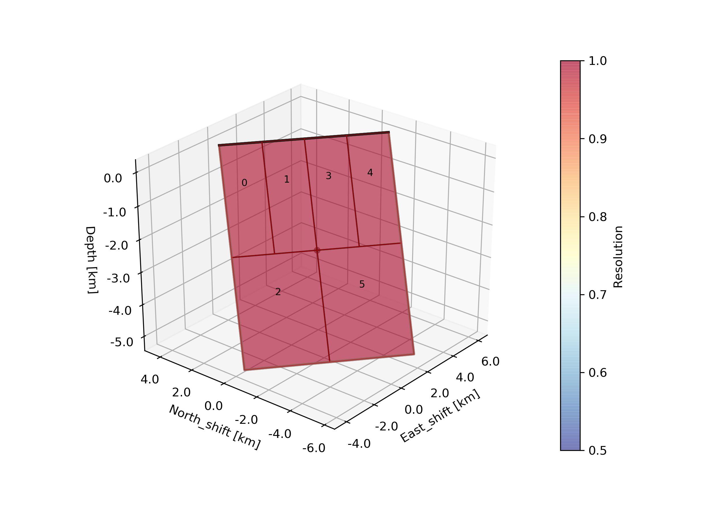
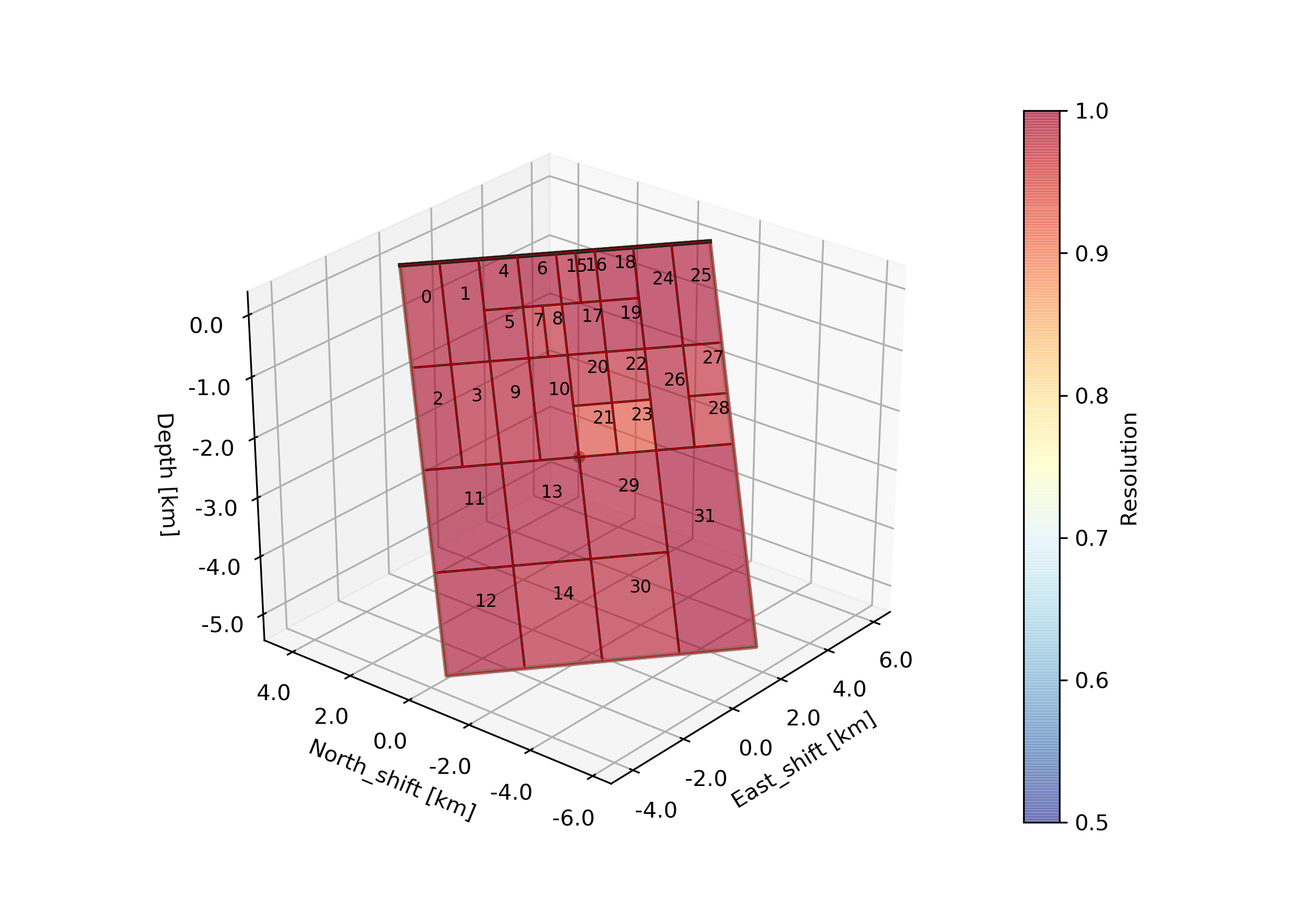
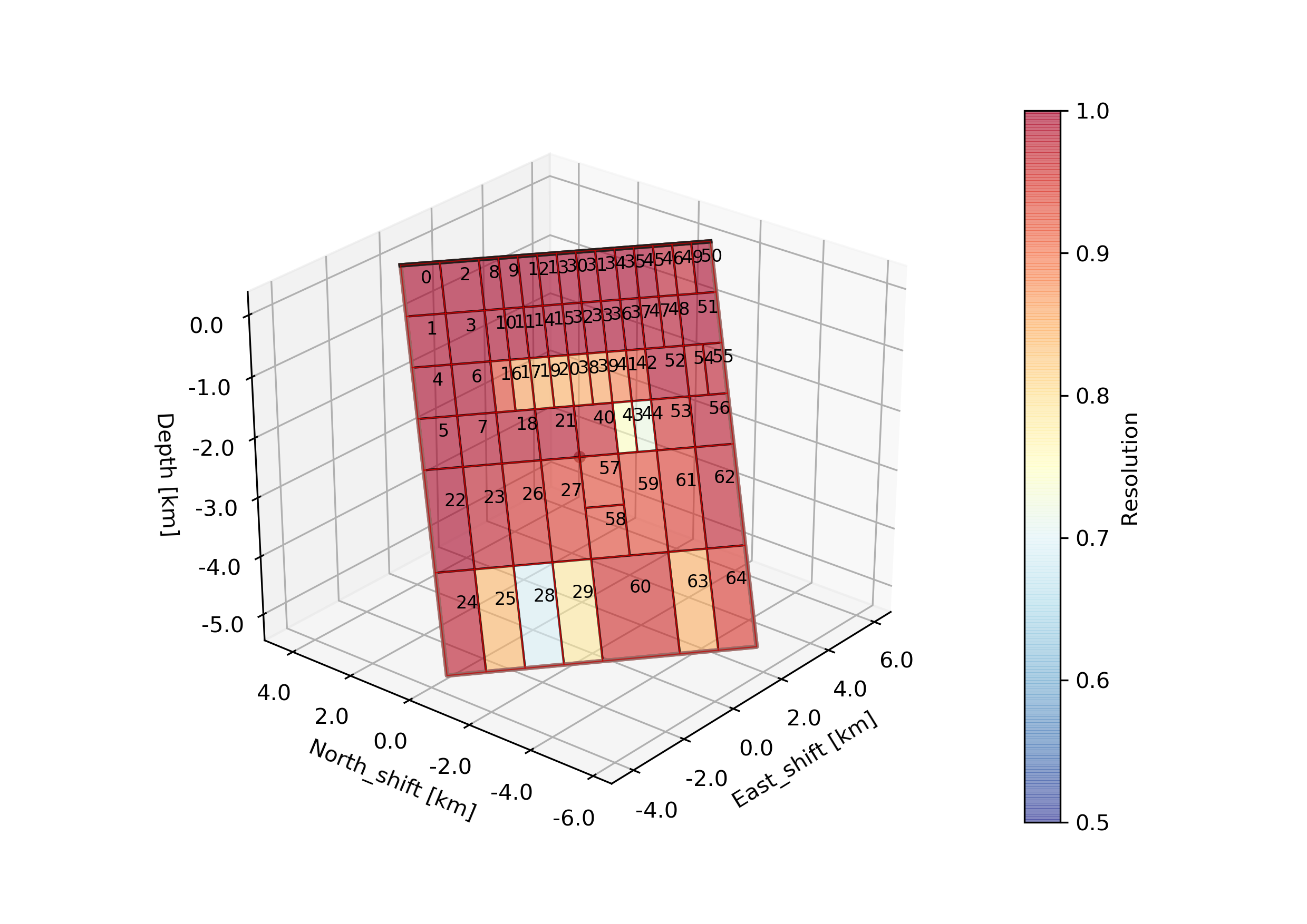
The –plot option creates a plot of the discretized dike geometry (under Fernandina/ffi/figures) with the individual patch resolutions. The higher the resolution the better the opening can be resolved. Also it will generate following trade-off curve showing the model resolution spread vs. epsilon [Atzori2019]. The black numbers indicate the corresponding number of patches.
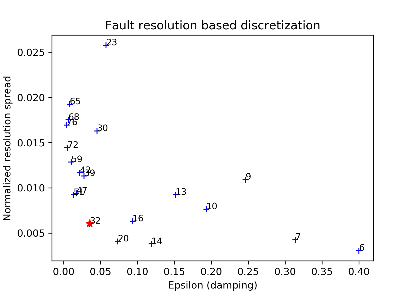
The fault/dike at the elbow of the trade-off curve (red star) will then be selected to run the sampling (middle). Also we see an over- and under-damped case top and bottom, respectively.
As we do have irregular patch sizes we cannot use the nearest_neighbor correlation_function for the Laplacian, but we use a gaussian instead. Please edit the file accordingly! The mode_config should look like this:
mode_config: !beat.FFIConfig
  regularization: laplacian
  regularization_config: !beat.LaplacianRegularizationConfig
    correlation_function: gaussian
  initialization: lsq
  npatches: 32
  subfault_npatches:
  - 32
Warning
The npatches and subfault_npatches argument were updated automatically and must not be edited by the user. These might differ slightly for the run of each user depending on the parameter configuration and as the discretization algorithm is not purely deterministic.
Manually selecting another fault discretizaion
It might happen that the user favors another discretization, instead of the one selected by the algorithm. Please see Example 4b for how to select another discretization.
Sample
Now the solution space can be sampled using following sampler configuration:
sampler_config: !beat.SamplerConfig
  name: SMC
  backend: bin
  progressbar: true
  buffer_size: 5000
  buffer_thinning: 40
  parameters: !beat.SMCConfig
    tune_interval: 50
    check_bnd: true
    rm_flag: false
    n_jobs: 4
    n_steps: 400
    n_chains: 1000
    coef_variation: 1.0
    stage: 0
    proposal_dist: MultivariateCauchy
    update_covariances: false
Note
For more detailed search of the solution space please modify the parameters ‘n_steps’ and ‘n_chains’ for the SMC sampler in the $project_directory/config_ffi.yaml file to higher numbers. Depending on these specifications and the available hardware the sampling may take several hours. Further remarks regarding the configuration of the sampler can be found here .
The sampling can be started with
beat sample Fernandina --mode=ffi
Summarize and plotting
After the sampling successfully finished, the final stage results have to be summarized with:
beat summarize Fernandina --stage_number=-1 --mode=ffi
After that several figures illustrating the results can be created. To create all available plots for the model setup run:
beat plot Fernandina_nosmooth all --mode=ffi --stage_number=-1 --nensemble=300
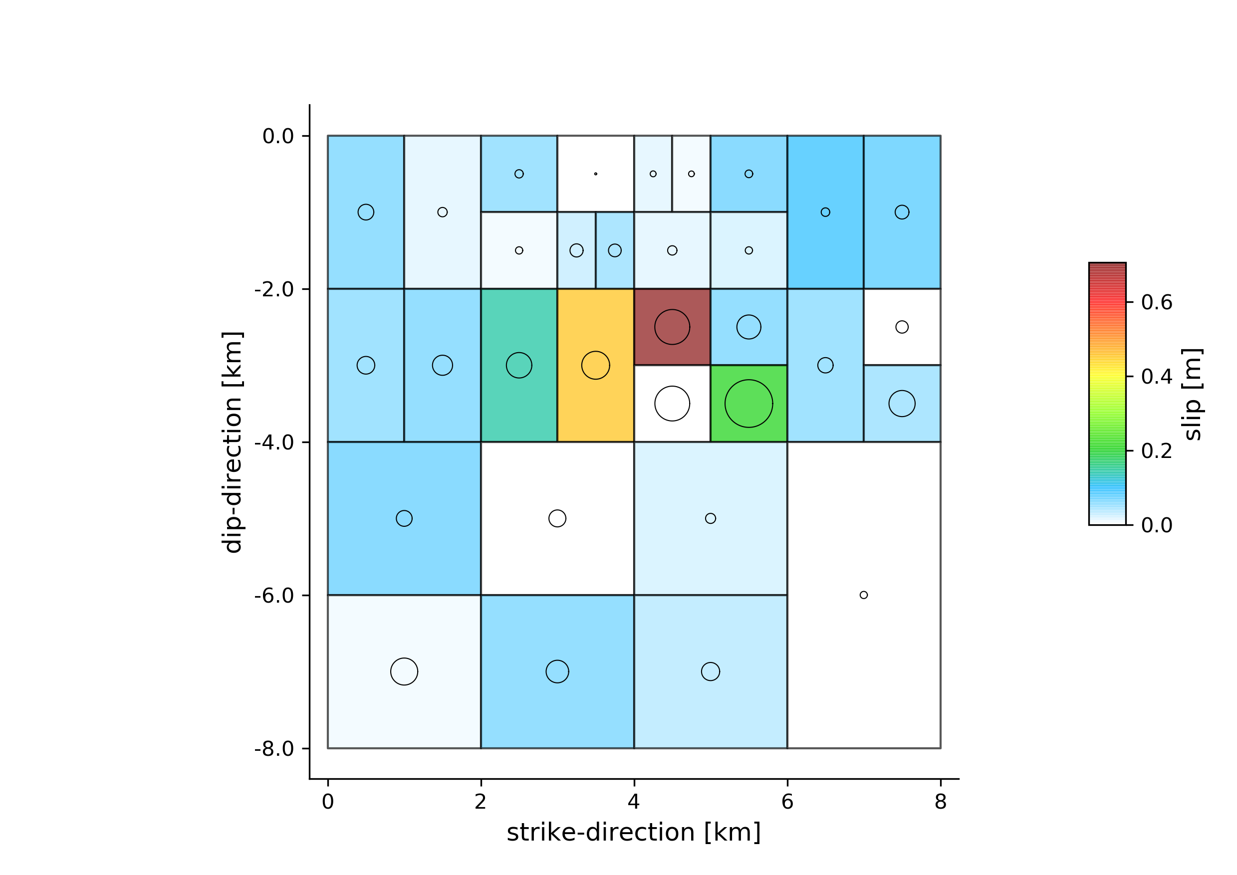
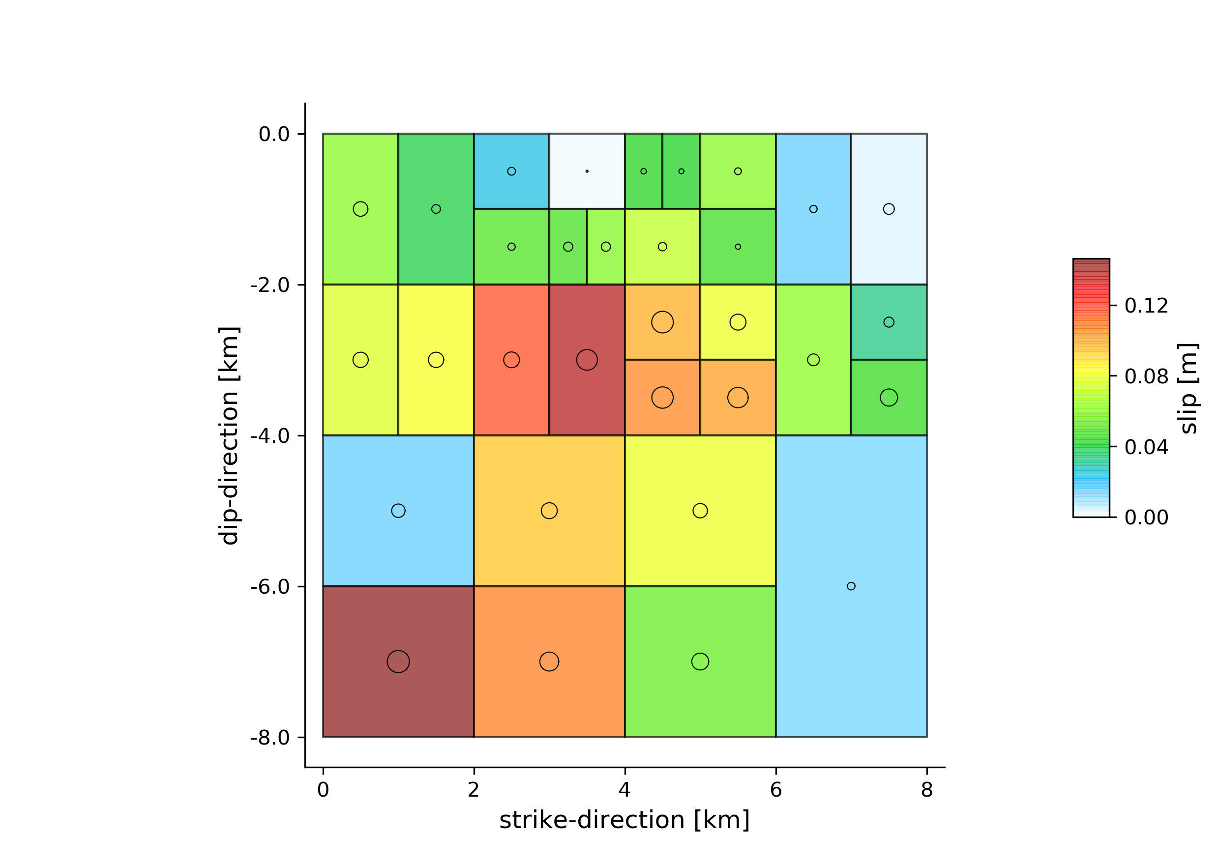
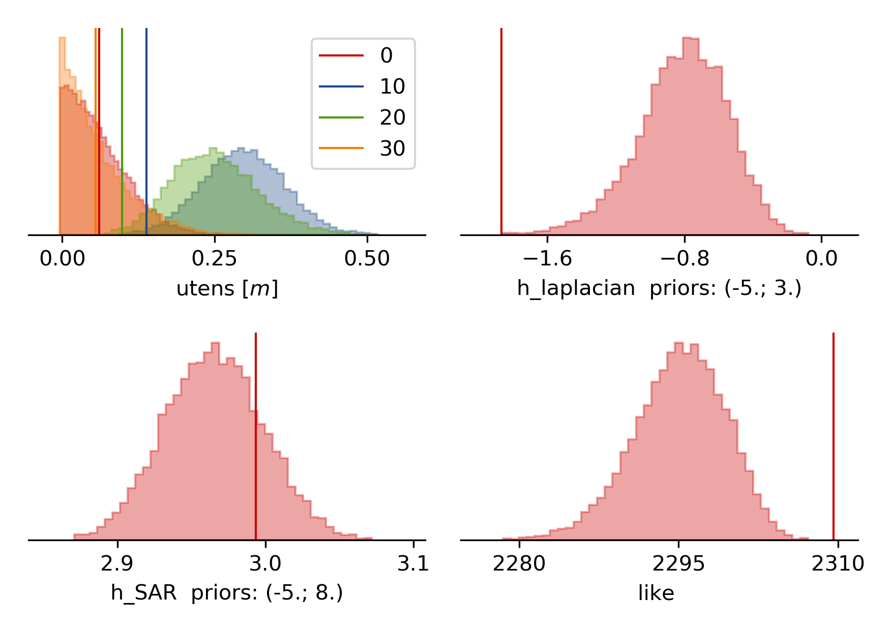
The slip-distribution:
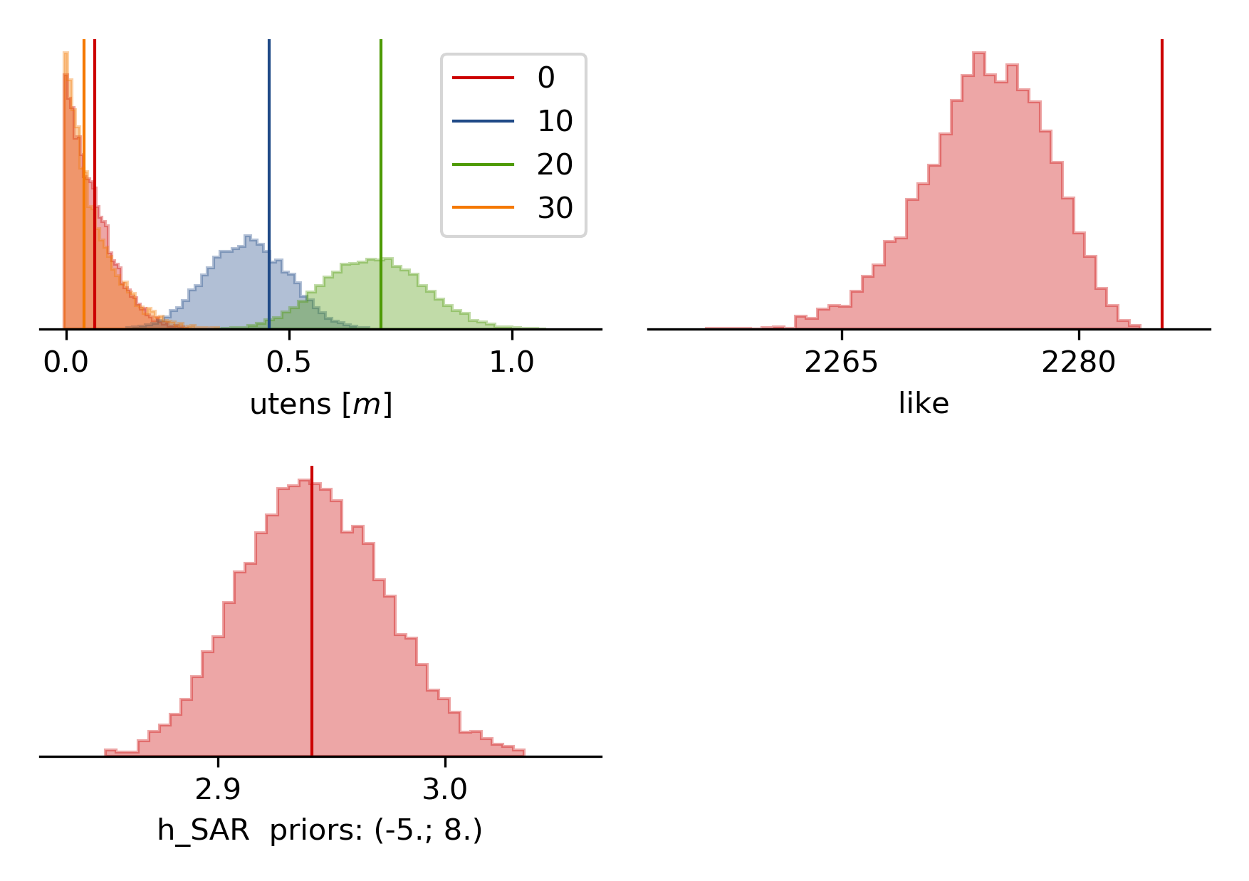
The histograms for the laplacian smoothing, the noise scalings and the posterior likelihood:
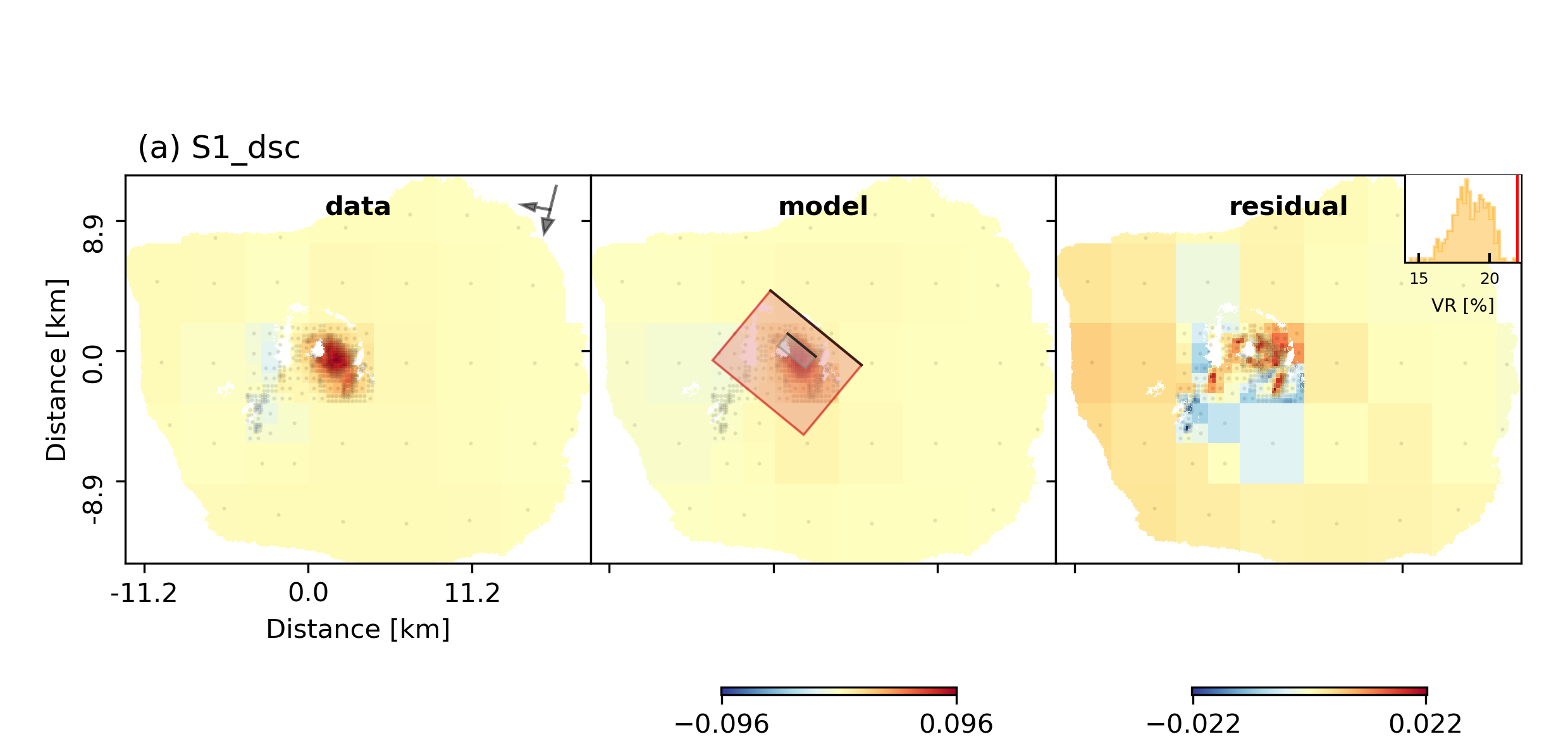
The comparison between data, synthetic displacements and residuals for the two InSAR tracks in a local coordinate system and a histogram of weighted variance reduction for a posterior model ensemble of 300 models:
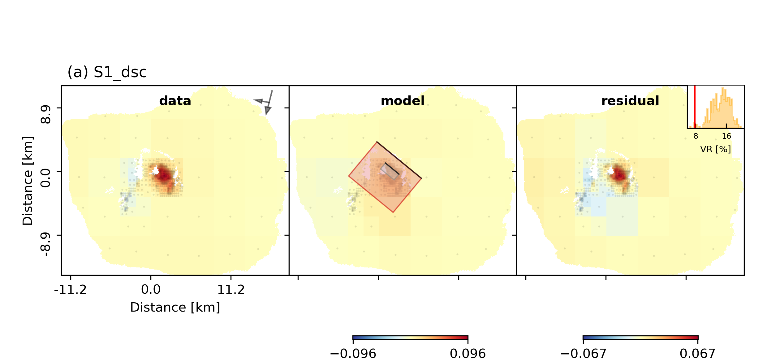
The plot should show something like this. Here the residuals are displayed with an individual color scale according to their minimum and maximum values.
Now we notice that the variance reductions are significantly worse than the uniform slip results (~5%) and there are large correlated residuals left. The maximum slip (opening~tensile slip) values in the slip distribution (i.e. opening distribution) are much less than the uniform slip that was inferred in example 6. The reason for this is that the Laplacian smoothing in this case did not allow for a small patch with large opening as this would not be considered “smooth” in the model!!!
So we want to rerun the model without Laplacian smoothing. This is possible, because we optimized the sizes of each patch to be still resolvable by the data with the “full resolution” algorithm [Atzori2011], [Atzori2019] and we likely did not overparameterize the dikes surface.
Clone setup and repeat sampling
We do not want to throw away the previous result, but we want to keep (almost) the same model setup. So we clone the setup and the data into a new directory “Fernandina_nosmooth”:
beat clone Fernandina Fernandina_nosmooth --mode=ffi --datatypes=geodetic --copy_data
To disable the laplacian smoothing we set the mode config to:
mode_config: !beat.FFIConfig
  regularization: none
  initialization: lsq
  npatches: 32
  subfault_npatches:
  - 32
Now we rerun the new setup without smoothing, summarize and plotting:
beat sample Fernandina_nosmooth --mode=ffi
beat summarize Fernandina_nosmooth --stage_number=-1 --mode=ffi
beat plot Fernandina_nosmooth all --mode=ffi --stage_number=-1 --nensemble=300
Now the datamisfits and opening distribution look much more reasonable: