Example 4b: Static finite-fault estimation, resolution based patch discretization

In this example we will determine a variable slip distribution for the L’aquila 2009 earthquake by using static InSAR data. In contrast to Example 4a we will use resolution based discretization of fault patches following the approach of [Atzori2011]. It is assumed that the reader has Example 4a completed before following this example, in order to be familiar with the concepts and commands for uniform discretized faults.

Clone

Please clone the config_ffi.yaml from the previous uniform static FFI run for the Laquila earthquake:

beat clone Laquila Laquila_resolution --mode=ffi --datatypes=geodetic --copy_data

Calculate Greens Functions

In the uniformly discretized fault variable slip estimation we did define the reference fault geometry based on the results of Example 3 where we did estimate the fault geometry parameters. Based on the reference fault and the available data observations the model resolution matrix can be calculated and the fault can be divided into patches such that a defined threshold of resolution is met. For details on the algorithm I refer the reader to the original article of [Atzori2011].

In this example we want to discretize the fault surface using such a resolution based discretization. Todo so, please set the discretization attribute of the gf_config to resolution and run the update command to display changes to the config:

beat update Laquila_resolution --mode=ffi --diff

Rerun without –diff to apply the changes:

beat update Laquila_resolution --mode=ffi

The discretization config should look now like this:

discretization: resolution
discretization_config: !beat.ResolutionDiscretizationConfig
  extension_widths:
  - 0.1
  extension_lengths:
  - 0.1
  epsilon: 0.004
  epsilon_search_runs: 1
  resolution_thresh: 0.999
  depth_penalty: 3.5
  alpha: 0.3
  patch_widths_min:
  - 1.0
  patch_widths_max:
  - 5.0
  patch_lengths_min:
  - 1.0
  patch_lengths_max:
  - 5.0

The patch sizes will be iteratively optimized to be between the min and max values in length and width. Starting from large patches at patch_widths_max and patch_lengths_max they will be divided into smaller pieces until the patches are either smaller/equal than the defined patch_widths_min and patch_lengths_min or if the patches resolution is below the defined resolution_thresh. The alpha parameter determines how many of the patch candidates to be divided further, are actually divided in the next iteration (0.3 means 30%). The epsilon parameter here is most important in determining the final number of patches. The higher it is, the smaller the number of patches is going to be. The depth_penalty parameter is set to a reasonable value and likely does not need to be touched. The higher it is, the larger the patches that are at larger depth are going to be.

For the Laquila case please set the following config attributes to:

Attribute name	Value
extension_width	0.4
extension_length	0.4
epsilon	0.004
epsilon_search_runs	15
alpha	0.1
patch_widths_min	1.0
patch_widths_max	25.0
patch_lengths_min	1.0
patch_lengths_max	25.0
depth_penalty	3.5

The nworkers attribute determines the number of processes to be run in parallel to calculate the Greens Functions and should be set to a sufficiently high number that the hardware supports (number of CPU -1).

With epsilon_search_runs we can control the number of models that are run automatically with different epsilon parameters on a sensible search bound, starting with epsilon as the lowest.

We can start the discretization optimization with:

beat build_gfs Laquila_resolution --mode=ffi --datetypes=geodetic --execute --force --plot

Note

The –force option is needed to overwrite the previously discretized fault object that was copied during the clone command above.

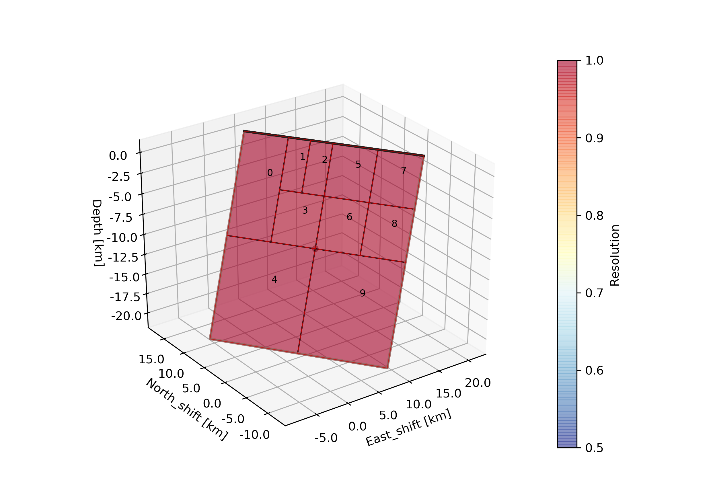
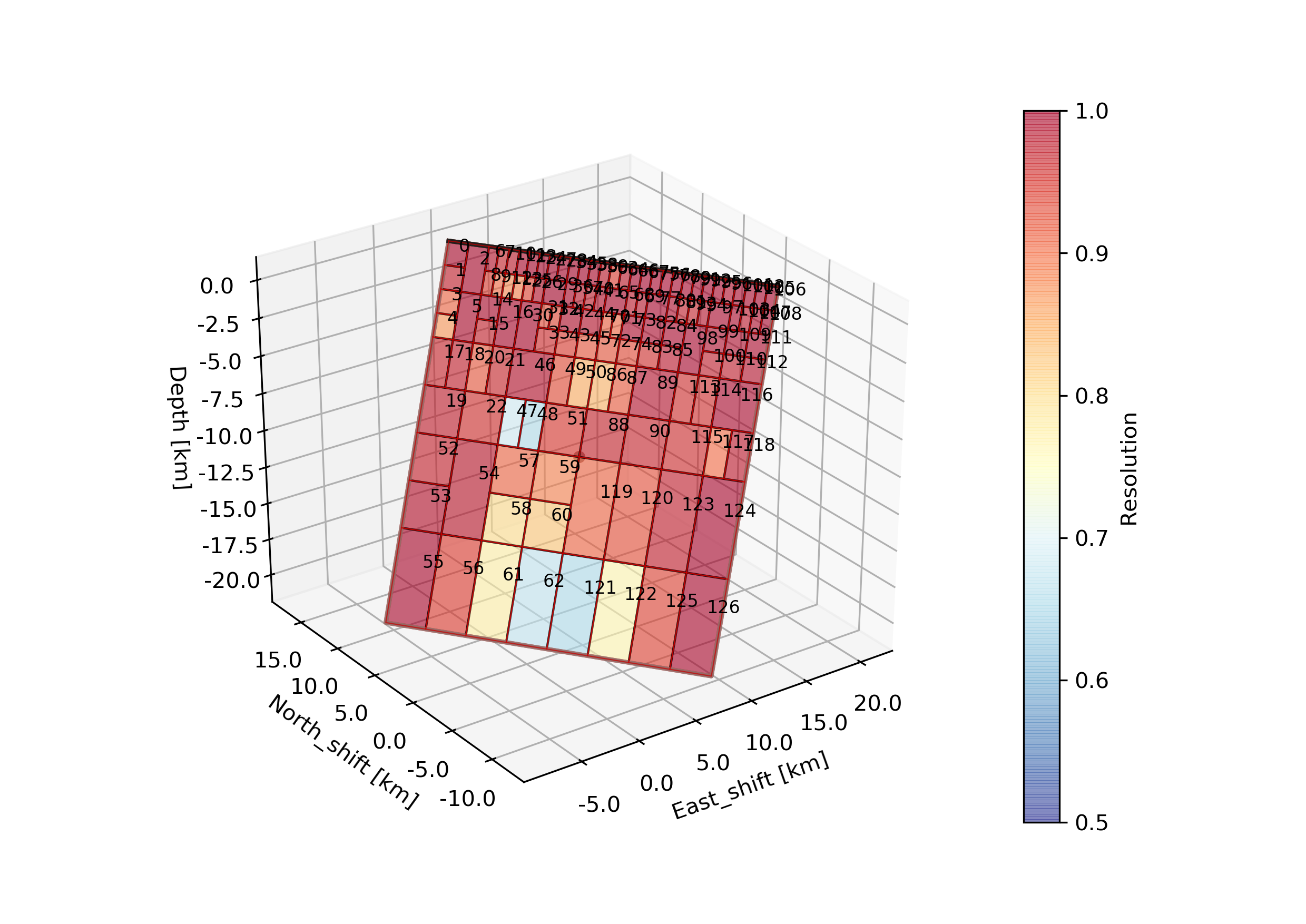
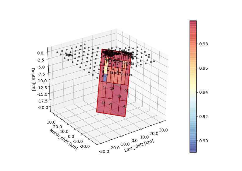
The –plot option creates a plot of the discretized fault geometry (under Laquila_resolution/ffi/figures) with the individual patch resolutions. The higher the resolution the better the slip can be resolved. Also it will generate following trade-off curve showing the model resolution spread vs. epsilon [Atzori2019]. The black numbers indicate the corresponding number of patches.

The fault at the elbow of the trade-off curve (red star) will then be selected to run the sampling (middle). Also we see an over- and under-damped case top and bottom, respectively.

As we do have irregular patch sizes we cannot use the nearest_neighbor correlation_function for the Laplacian, but we use a gaussian instead. Please edit the file accordingly! The mode_config should look like this:

mode_config: !beat.FFIConfig
  regularization: laplacian
  regularization_config: !beat.LaplacianRegularizationConfig
    correlation_function: gaussian
  initialization: lsq
  npatches: 119
  subfault_npatches:
  - 119

Warning

The npatches and subfault_npatches argument were updated automatically and must not be edited by the user. These might differ slightly for the run of each user depending on the parameter configuration and as the discretization algorithm is not purely deterministic.

Manually selecting another fault discretizaion

It might happen that the user favors another discretization, instead of the one selected by the algorithm. All the discretized fault objects (each indicated by the respective epsilon suffix) are stored under:

Laquila_resolution/ffi/linear_gfs/discretization

The fault_geometry, which is used for sampling is stored under:

Laquila_resolution/ffi/linear_gfs/discretization/fault_geometry.pkl

In our case here the user might favor for example the fault that was discretized with 42 patches instead of the selected solution with 28 patches, because it potentially allows to sample finer features of the slip distribution. In our case the fault with 42 patches has an epsilon value of ca. 0.05. Checking the discretization directory with:

ls Laquila_resolution/ffi/linear_gfs/discretization/

We can identify the fault object to be:

fault_geometry_0.0555798197749255.pkl

We copy that to the destination of the sampled fault geometry:

cp Laquila_resolution/ffi/linear_gfs/discretization/fault_geometry_0.0555798197749255.pkl Laquila_resolution/ffi/linear_gfs/fault_geometry.pkl

The following command allows to double-check the chosen patch discretization.:

beat check Laquila_resolution --mode=ffi --what=discretization

Now the linear Greens Functions need to be recalculated for that chosen fault geometry.:

beat build_gfs Laquila_resolution --mode=ffi --datatypes=geodetic --execute

Sample

Now the solution space can be sampled using the same sampler configuration as for example 4a, but with the resolution based fault discretization:

beat sample Laquila_resolution --mode=ffi

Warning

Please be aware that if the full kinematic model setup is planned to be run after the variable static slip estimation, the resolution based discretization cannot be used in its implemented form as the algorithm only works for static surface data.

Summarize and plotting

After the sampling successfully finished, the final stage results have to be summarized with:

beat summarize Laquila_resolution --stage_number=-1 --mode=ffi

After that several figures illustrating the results can be created.

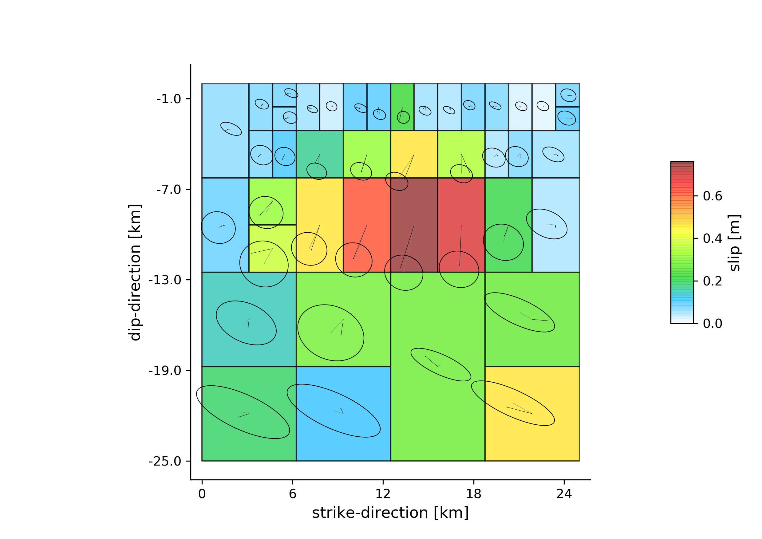
For the slip-distribution please run:

beat plot Laquila_resolution slip_distribution --mode=ffi

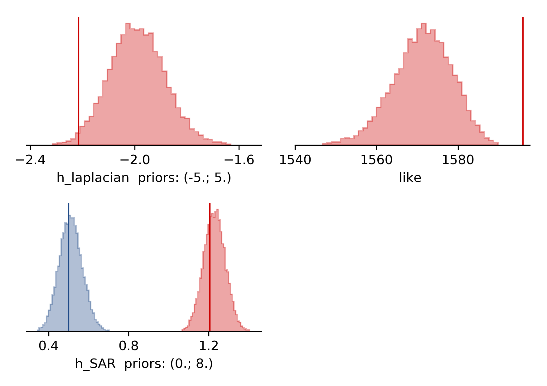
To get histograms for the laplacian smoothing, the noise scalings and the posterior likelihood please run:

beat plot Laquila_resolution stage_posteriors --stage_number=-1 --mode=ffi --varnames=h_laplacian,h_SAR,like

For a comparison between data, synthetic displacements and residuals for the two InSAR tracks in a local coordinate system and a histogram of weighted variance reduction for a posterior model ensemble of 200 models please run:

beat plot Laquila_resolution scene_fits --mode=ffi --nensemble=200

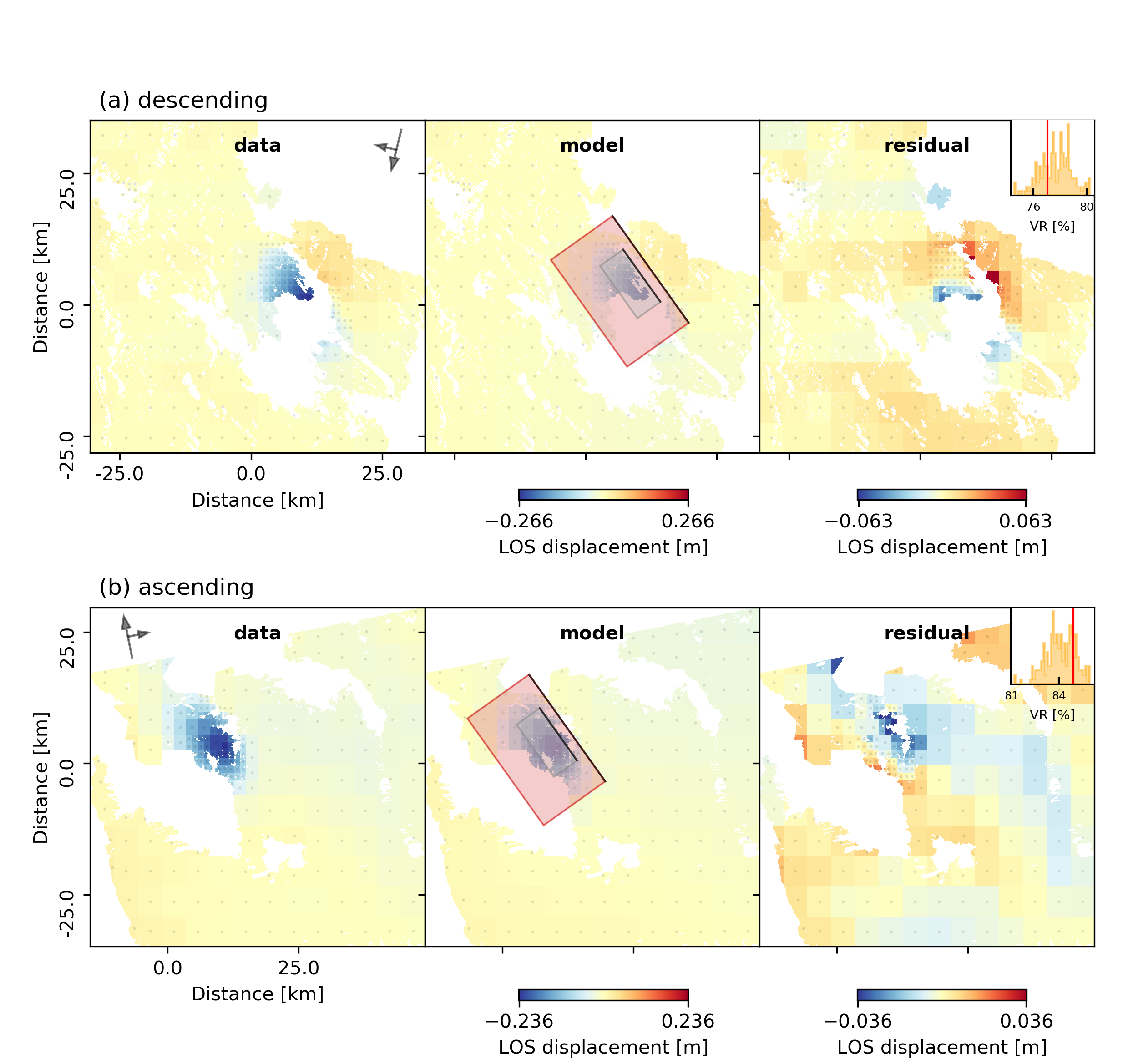
The plot should show something like this. Here the residuals are displayed with an individual color scale according to their minimum and maximum values.

References

[Atzori2011] (1,2)

Atzori, S. and Antonioli, A. (2011). Optimal fault resolution in geodetic inversion of coseismic data Geophys. J. Int. (2011) 185, 529–538, link

[Atzori2019]

Atzori, S.; Antonioli, A.; Tolomei, C.; De Novellis, V.; De Luca, C. and Monterroso, F. InSAR full-resolution analysis of the 2017–2018 M > 6 earthquakes in Mexico Remote Sensing of Environment, 234, 111461,