
Fomosto tutorial
Fomosto is a tool to help create and work with pre-calculated and stored Green’s functions.
Introduction
Many seismological methods require knowledge of Green’s functions in dependance of ranges of source and receiver coordinates. Examples range from synthetic seismogram calculation over source imaging techniques to source inversion methods. Calculation of Green’s functions is a computationally expensive operation and it can be of advantage to calculate them in advance. The same Green’s function traces can then be reused several or many times as required in a typical application.
Regarding Green’s function creation as an independent step in a use-case’s processing chain encourages the storage of these in an application independant form. They can then immediatly be reused when new data is to be processed, they can be shared between different applications and they can also be passed to other researchers, allowing them to focus on their own application rather then spending days of work to get their Green’s function setup ready.
Furthermore, it is useful to store associated meta information, like e.g. travel time tables for seismic phases and the earth model used, together with the Green’s function in order to have a complete and consistent framework to play with.
Pyrocko contains a flexible framework to store and work with pre-calculated
Green’s functions. It is implemented in the pyrocko.gf subpackage.
Also included, is a powerful front end tool to create, inspect, and manipulate
Green’s function stores: the fomosto tool (”forward model storage
tool”).
Invocation and online help
Fomosto is a command line program. A brief help overview is shown, when it is started without any arguments.
- fomosto
- fomosto server
$ fomosto
Usage: fomosto <subcommand> <arguments> ... [options]

Subcommands:

    init          create a new empty GF store
    build         compute GFs and fill into store
    stats         print information about a GF store
    check         check for problems in GF store
    decimate      build decimated variant of a GF store
    redeploy      copy traces from one GF store into another
    view          view selected traces
    extract       extract selected traces
    import        convert Kiwi GFDB to GF store format
    export        convert GF store to Kiwi GFDB format
    ttt           create travel time tables
    tttview       plot travel time table
    tttextract    extract selected travel times',
    server        run seismosizer server,
    download      download GF store from a server,
    modelview     plot earthmodels,
    upgrade       upgrade store format to latest version,
    addref        import citation references to GF store config,
    qc            quality check,
    report        report for Green's function databases,

To get further help and a list of available options for any subcommand run:

    fomosto <subcommand> --help
The first argument selects the subcommand. All other arguments and options are
dependant on the subcommand. Options start with a double dash, as in
--option. If an option takes an argument, it must immediatly follow the
option, as in --option=argument.
Creating a new Green’s function store
Fomosto does not do the actual computation of the Green’s functions. A separate Green’s function modelling code is required to do this.
However, Fomosto provides a unified interface to configure and run these codes in order to make it simple to build a database of pre-calculated Green’s functions.
Four modelling codes, including Python interfaces required for Fomosto are hosted in the Pyrocko code repository:
For detailled information regarding each computation code refer to the
Downloads/Software website of section 2.1 (GFZ): https://www.gfz-potsdam.de/en/section/physics-of-earthquakes-and-volcanoes/infrastructure/tool-development-lab.
Green’s function stores calculated with QSSP and QSEIS can be used for dynamic waveform and static displacement modeling. Green’s functions stores which are created with the PSGRN-PSCMP backend return step functions and are therefore mostly applicable to static displacement
modeling.
Installation is done for each code inside the uncompressed folder by (More information in each packages’ README.md):
qseis¶autoreconf -i # only if 'configure' script is missing
./configure
make
sudo make install
In this example, we will use QSEIS as the modelling code.
To initialize an empty Green’s function store to be built with QSEIS 2006b run:
$ fomosto init qseis.2006b my_first_gfs
to use a different backend, e.g. QSSP 2010, run:
$ fomosto init qssp.2010 my_first_gfs
A directory named my_first_gfs, containing some example configuration files
is created:
my_first_gfs/
|-- config       # (1)
`-- extra/
    `-- qseis    # (2)
The file config (1) contains general settings and the file extra/qseis
(2) contains extra settings which are specific to the QSEIS modelling code.
These files are in the YAML format, which is a good
compromise between human and computer readability. The contents of the
configuration files are disussed in the next section. The default
configuration produced by the fomosto init command can be used without any
modifications for a quick functional test.
First step is to create tabulated phase arrivals:
$ cd my_first_gfs
$ fomosto ttt
...
$ ls phases/
begin.phase  end.phase  p.phase  P.phase  s.phase  S.phase
These tabulated phase arrivals are later, in the build step, used to cut the generated Green’s function traces before insertion into the database.
Now, we can calculate the Green’s function traces:
$ fomosto build
Green’s functions are built in parallel, if possible. The number of worker processes
may be limited with the --nworkers=N option.
We now have a complete Green’s function store, ready to be used. This is the directory structure of the store:
my_first_gfs/         # this directory represents the GF store
|-- config            # general settings
|-- decimated/        # directory for decimated variants of the store
|-- extra/            # any extra meta information is in here
|   `-- qseis         # e.g. parameters used for the initial modelling
|-- index             # index part of the storage
|-- phases/           # tabulated phase arrivals are looked for in here
|   |-- begin.phase
|   |-- end.phase
|   |-- p.phase
|   |-- P.phase
|   |-- s.phase
|   `-- S.phase
`-- traces            # big binary file with the actual GF data samples
We may now want to change some configuration values and rebuild the Green’s functions.
Configuration
These are the initial contents of the config file:
--- !pyrocko.gf.meta.ConfigTypeA  # this type is for cylindrical symmetry with
                                  # receivers all at the same depth

# this label should be set to something unique if the GF store should be published
id: my_qseis_gf_store

# indicates, that QSEIS is/was used for the modelling
modelling_code_id: qseis

# a layered earth model, used for modelling of the Green's functions
# and for calculation of phase arrivals. Format is the 'nd' format
# as used in cake.

earthmodel_1d: |2  # '|2' means that a text block indented with 2 blanks follows
      0.             5.8            3.46           2.6         1264.           600.
     20.             5.8            3.46           2.6         1264.           600.
     20.             6.5            3.85           2.9         1283.           600.
     35.             6.5            3.85           2.9         1283.           600.
  mantle
     35.             8.04           4.48           3.58        1449.           600.

     ...

sample_rate: 0.2  # [Hz] or [days] for PSGRN/PSCMP
ncomponents: 10   # number of Green's function components (always use 10 with QSEIS).

# travel time tables are calculated for the phase arrivals defined below
# the travel time tables can be referenced at other points in the configuration
# by their id
tabulated_phases:
- !pyrocko.gf.meta.TPDef
  id: begin
  definition: p,P,p\,P\,Pv_(cmb)p     # phase defintions in *cake* syntax, first available arrival is used
- !pyrocko.gf.meta.TPDef
  id: end
  definition: '2.5'                   # this simply means 2.5 km/s horizontal velocity
- !pyrocko.gf.meta.TPDef
  id: P
  definition: '!P'                    # exclamation mark: a *cake classic phase name* follows

  ...

# uniform receiver depth with this type of GF config
receiver_depth: 0.0  # [m]

# extents and spacing of the GF traces [m]
source_depth_min: 10000.0
source_depth_max: 20000.0
source_depth_delta: 10000.0
distance_min: 100000.0
distance_max: 1000000.0
distance_delta: 10000.0
Details about the structures in the config file are given in the
documentation of the pyrocko.gf.meta module. In this case, e.g. see
the class pyrocko.gf.meta.ConfigTypeA.
The initial contents of the QSEIS specific configuration file extra/qseis:
--- !pyrocko.fomosto.qseis.QSeisConfig #

# with the folowing setting, Green's functions will be calculated for (at
# least) the time region between  'begin' minus 50 seconds to 'end' plus 100
# seconds, where 'begin' and  'end' are tabulated phases as defined in the
# main configuration

time_region: [begin-50, end+100]  # see note below

# cut the Green's functions to the same time span

cut: [begin-50, end+100]  # see note below

# following docs are excerpts from the QSEIS documentation

# select slowness integration algorithm (0 = suggested for full wave-field
# modelling; 1 or 2 = suggested when using a slowness window with narrow
# taper range - a technique for suppressing space-domain aliasing)

sw_algorithm: 0

# 4 parameters for low and high slowness (Note 1) cut-offs [s/km] with
# tapering: 0 < slw1 < slw2 defining cosine taper at the lower end, and 0 <
# slw3 < slw4 defining the cosine taper at the higher end. default values
# will be used in case of inconsistent input of the cut-offs (possibly with
# much more computational effort)

slowness_window: [0.0, 0.0, 0.0, 0.0]    # [s/km]

# parameter for sampling rate of the wavenumber integration (1 = sampled
# with the spatial Nyquist frequency, 2 = sampled with twice higher than
# the Nyquist, and so on: the larger this parameter, the smaller the space-k

wavenumber_sampling: 2.5

# the factor for suppressing time domain aliasing (> 0 and <= 1) The
# suppression of the time domain aliasing is achieved by using the complex
# frequency technique. The suppression factor should be a value between 0 and
# 1. If this factor is set to 0.1, for example, the aliasing phase at the
# reduced time begin is suppressed to 10%.

aliasing_suppression_factor: 0.1

# switch for filtering free surface effects (0 = with free surface, i.e.,
# do not select this filter; 1 = without free surface; 2 = without free
# surface but with correction on amplitude and wave form. Note switch 2
# can only be used for receivers at the surface)

filter_surface_effects: 0

# switch for filtering waves with a shallow penetration depth (concerning
# their whole trace from source to receiver), penetration depth limit [km]
# if this option is selected, waves whose travel path never exceeds the
# given depth limit will be filtered ("seismic nuting"). the condition for
# selecting this filter is that the given shallow path depth limit should
# be larger than both source and receiver depth.

filter_shallow_paths: 0
filter_shallow_paths_depth: 0.0  # [km]

# switch for flat-earth-transform

sw_flat_earth_transform: 1

# gradient resolution [%] of vp, vs, and density, if <= 0, then default
# values (depending on wave length at cut-off frequency) will be used

gradient_resolution_vp: 0.0
gradient_resolution_vs: 0.0
gradient_resolution_density: 0.0

# wavelet duration [unit = time sample rather than sec!], that is about
# equal to the half-amplitude cut-off period of the wavelet (> 0. if <= 0,
# then default value = 2 time samples will be used)

wavelet_duration_samples: 0.001

# switch for the wavelet form (0 = user's own wavelet; 1 = default wavelet:
# normalized square half-sinusoid for simulating a physical delta impulse;
# 2 = tapered Heaviside wavelet, i.e. integral of wavelet 1)

wavelet_type: 2
Note
The syntax for the timings in the time_region and cut in the above
example configuration is described in pyrocko.gf.meta.Timing.
If configuration values have been changed, it may be neccessary to rebuild the
tabulated phase arrivals or the Green’s functions. By default, Fomosto will
refuse to overwrite any GF store content. Use the --force option to override
this behaviour:
$ fomosto ttt --force
$ fomosto build --force
When debugging problems with the GF modelling setup, it can be helpful to increase the verbosity of the program:
$ fomosto build --loglevel=debug --nworkers=1
This will show in more detail, e.g. what input is generated for the modelling code.
Considerations for real-world applications
A Green’s function store of type A (pyrocko.gf.meta.ConfigTypeA)
contains precalculated Green’s functions on a grid for combinations of source
depth z and source-receiver surface distance x. How many Green’s functions
to calculate in advance is determined by the use-case. The depth range to be
calculated is given by the earthquake source depths to be studied. The distance
range by the smallest and largest distances between possible source points and
receiver positions. How dense the grid has to be made depends on whether we
want to be able to later interpolate the Green’s function between neighboring
nodes (a requirement for the analysis of extended sources) or if we don’t have
such a requirement. For bilinear interpolation to work fine, it is neccessary
to make the grid dense enough, so that no aliasing effects can occur. This
means that the grid spacing dx should be (considerably) smaller than v_min /
f_max, where v_min is the slowest apparent velocity of the seismic waves at
the surface and f_max is the highest frequency to be analysed. For example if
we want to study waveforms in a frequency range of up to 2 Hz and the slowest
horizontal velocities are 2 km/s, we need a grid spacing well below 1 km so we
may try with 250 m. The Green’s functions should be calculated with a temporal
sampling rate of at least 4 Hz in this example, better more.
Typically there is some trial and error involved in determining a stable and efficient set of parameters for a new modelling setup. The strategy is to first do some trial runs with a sparse grid and/or with a lowered sampling rate until we get a feeling for the modelling parameters. The final run for a dense grid, may take days or even weeks of computation time and we don’t want to waste that effort.
Diagnostics
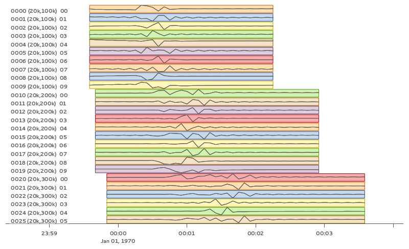
To quickly visualize selected Green’s function traces use Fomosto’s view subcommand. Run the following command to show the Green’s function traces for ten equally spaced distances:
$ fomosto view --extract='20k,@10'
If we are not in the Green’s function store’s directory, we can equally use:
$ fomosto view --extract='20k,@10' path/to/my_first_gfs
The extracted traces are shown in a Snuffler window, labeled as <counter>
(<source-depth>, <distance>) <component>.
It is also possible to directly compare the traces of two (or more) different
Green’s function stores. As a demonstration, here we created two Green’s
function stores, one using QSEIS for the modelling (qseis-test), the other
using QSSP (qssp-test). The example configurations produced by fomosto
init ... have been used, only the sampling rate has been changed to 1 Hz in
both. To compare some traces of the two Green’s function stores append both
their directory names to the view command:
$ fomosto view qseis-test qssp-test --extract='20k,@5'
Rearranging the view in Snuffler a bit, we can quickly spot some differences:
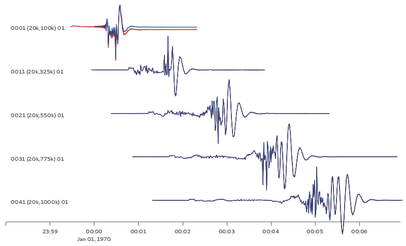
Here we can see, that at the closest distance, the QSEIS trace (red) contains a final static offset, while the QSSP trace (blue) does not.
Other diagnostic subcommands are fomosto tttview to visualize the travel
time tables, fomosto stats to summarize some technical details, and
fomosto check which checks the store for NaN values and some other
problems.
Report subcommand
The report subcommand will create a pdf document containing an artefacts report, displacement seismograms, velocity seismograms (optional), maximum amplitude graphs for seismograms, spectrum graphs, earth model graphs and the contents of the Green’s function configuration file. Each set of seismograms will contain five graphs with increasing amplitude scales. To view the subcommands of report, it can be ran without any arguments from the command line.
$ fomosto report
Create a pdf of displacment and velocity traces, max. amplitude of traces
and displacment spectra for Green's function stores.

Usage: fomosto report <subcommand> <arguments> ... [options]

Subcommands:

    single          create pdf of a single store
    double          create pdf of two stores
    sstandard       create a single store pdf with standard setup
    dstandard       create a double store pdf with standard setup
    slow            create a single store pdf, filtering the
                    traces with a low frequency
    dlow            create a double store pdf, filtering the
                    traces with a low frequency
    shigh           create a single store pdf, filtering the
                    traces with a low frequency
    dhigh           create a single store pdf, filtering the
                    traces with a low frequency
    slowband        create a single store pdf with a low
                    frequency band filter
    dlowband        create a double store pdf with a low
                    frequency band filter
    shighband       create a single store pdf with a high
                    frequency band filter
    dhighband       create a double store pdf with a high
                    frequency band filter
    snone           create a single store pdf with unfiltered traces
    dnone           create a double store pdf with unfiltered traces

To get further help and a list of available options for any subcommand run:

    fomosto report <subcommand> --help
Configuration file for Report subcommand
Here is a minimal configuration file (to be used with the fomosto report single command). If wanting to use the fomosto report double command, just copy/paste the entire contents below the existing contents, and change only the store_dir path. To see a full configuration file, use the output option on any of the fomosto report subcommands.
--- !gft.GreensFunctionTest  # this line is a must

# needs to point to the main directory of the Green's function store
store_dir: /home/willey/src/gf_stores/iceland_reg_v2

# optional: these will base the applied filters on the sampling rate
# of the store
rel_lowpass_frequency: 0.125
rel_highpass_frequency: 0.25

# optional: these will set the absolute frequencys of the applied filters
# if neither are set, then the seismograms will not be filtered
# only one option can be used for low/highpass frequency, so if absolute
# frequencies are desried, comment/delete the above and uncomment those below
# lowpass_frequency: 0.0014
# highpass_frequency: 0.0018

# a section for the source objects to be used when creating seismograms
sources:

  # <name>: <type>, the specific source objects to be used, where the names
  # have to be unique (see pyrocko for available source objects
  # :py:class:`pyrocko.gf.seismosizer.Source`)
  source1: !pf.DCSource
    depth: 6500.0
    strike: -90.0
    dip: 90.0
    rake: -90.0

# a section for the sensor array objects to be used when creating seismograms
sensors:

  # <name>: !gft.SensorArray, where the name has to be unique
  sensors1: !gft.SensorArray
    depth: 0.0

    # these are the codes for the type of sensors (pyrocko.gf.Target objects)
    codes: ['', STA, '', R]

    # this is the direction [deg] in which the sensor monitors
    azimuth: 0.0

    # this the dip [deg] of the sensor
    dip: 0.0

    # minimum/maximum distances [m] for the sensorys to be array at
    distance_min: 1000.0
    distance_max: 500000.0

    # the direction [deg] along which the sensors will be arrayed
    strike: 0.0

    # amount of sensors per array
    sensor_count: 50
If there are multiple source and sensor array objects in the configuration file, then the command will create seismograms for every combination of source and sensor arry. Example (partial file):
sources:
  source1: !pf.DCSource
    depth: 6500.0
    strike: -90.0
    dip: 90.0
    rake: -90.0
  source2: !pf.DCSource
    depth: 6500.0
    strike: 45.0
    dip: 90.0
    rake: 180.0

sensors:
  sensors1: !gft.SensorArray
    depth: 0.0
    codes: ['', STA, '', R]
    azimuth: 0.0
    dip: 0.0
    distance_min: 1000.0
    distance_max: 500000.0
    strike: 0.0
    sensor_count: 50
  sensors2: !gft.SensorArray
    depth: 0.0
    codes: ['', STA, '', Z]
    azimuth: 0.0
    dip: 90.0
    distance_min: 1000.0
    distance_max: 500000.0
    strike: 0.0
    sensor_count: 50
This configuration file will create four sets of seismograms (source1-sensors1, source1-sensor-2, …), but if you only specific source-sensor array combinations, then use the optional parameter trace_configs like:
trace_configs:
- [source1, sensors2]
- [source2, sensors1]
placed at the bottom of the configuration file. This will only produce the seismograms for the listed combinations.
To try the configuration file, save to your home directory as min_config. Make sure you have the specified Green’s function store accessible. Then run:
$ fomosto report single ~/min_config
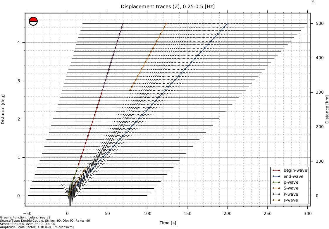
and you will create a pdf file called iceland_reg_v2_0.25-0.5Hz.pdf in your home directory. If you want to see what an output configuration file looks like:
$ fomosto report single ~/min_config --output=~/min_config_full
A example displacement seismogram.
Creating decimated variants of a Green’s function store
For some applications, it can be useful if the sampling rate of the Green’s functions are variable; for example if the method first analyses the lower frequency content of the signal and in a later stage refines the results including higher frequencies or if the frequency range to be analysed is dependant on the magnitude of the source. Because a lower sampling rate typically also means that the Green’s functions are required on a less dense spacial grid, this can lead to less computational effort and lower memory consumption of the application.
We can create downsampled variants of a Green’s function store with the
fomosto decimate command. For example, running
$ fomosto decimate 2
$ fomosto decimate 4
in a store directory creates variants of the database with half and a quater of
the original sampling rate. The downsampled variants are stored in the
decimated subdirectory of the store, so we can again compare the traces
with
$ fomosto view . decimated/2 decimated/4 --extract='@2,@5'
If not only the temporal but also the spacial sampling should be reduced, a modified configuration for the downsampled variants can be used:
$ cp config config.2.temp
$ # edit config2.temp; e.g. double the distance_delta value
$ fomosto decimate 2 --config=config.2.temp
$ rm config.2.temp
How to combine or split Green’s function stores
Sometimes, it is neccessary to combine or split Green’s function stores. For example if we want to extend an existing store with more additional source depths, or if we wish to extract a subset of an existing database. This is done with Fomosto by creating an empty target store with the desired extents and by then copying the relevant traces from the source stores to the target store.
Create empty copy of
my_first_gfs:$ fomosto init redeploy my_first_gfs derived
Adjust parameters in
derived/config; e.g. change the extents of the store.Copy traces from
my_first_gfstoderived. Only traces at nodes which are present in both stores are copied.$ fomosto redeploy my_first_gfs derived
Download pre-calculated Green’s function stores
Pre-calculated Green’s functions stores with global or regional coverage can be explored online at: