

Squirrel - Data access infrastructure
The Squirrel framework provides a unified interface to query and access seismic waveforms, station meta-data and event information from local file collections and remote data sources. For prompt responses, a database setup is used under the hood. To speed up assemblage of ad-hoc data selections, files are indexed on first use and the extracted meta-data is remembered for subsequent accesses. Bulk data is lazily loaded from disk and remote sources, just when requested. Once loaded, data is cached in memory to expedite typical access patterns. Files and data sources can be dynamically added and removed at run-time.
Features
Efficient (O log N) lookup of data relevant to a time window of interest.
Metadata caching and indexing.
Modified files are re-indexed as needed.
SQL database (sqlite) is used behind the scenes.
Can handle selections with millions of files.
Data can be added and removed at run-time, efficiently (O log N).
Just-in-time download of missing data.
Disk-cache of meta-data query results with expiration time.
Efficient event catalog synchronization.
Always-up-to-date data coverage indices.
Always-up-to-date indices of available station/channel codes.
Documentation and tutorials
The Squirrel framework consists of a library (subpackage
pyrocko.squirrel) and a front-end command line tool (executable
squirrel). For each of these, documentation and a tutorial is provided:
Additionally the concept of the framework is laid out in the following section.
Conceptual overview
This section provides a high level introduction to the Squirrel data access infrastructure by illustrating its basic functionality. For a more in-depth introduction, please refer to the tutorials listed above.
Environment
Import the framework and create a Squirrel instance:
from pyrocko import squirrel
sq = squirrel.Squirrel()
On the very first instantiation of a
Squirrel object, a new and initially empty
Squirrel environment
is created on disk (Fig. 1).
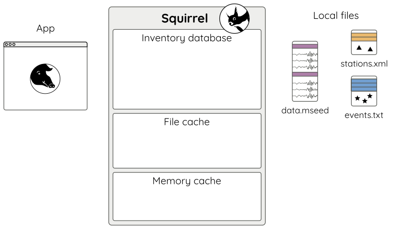
Figure 1: Fresh empty Squirrel environment.
The Squirrel environment sits between the application and the data holdings. It
consists of an SQLite database and caches. The environment is automatically
created when the first Squirrel instance is initialized. By default it is
stored in the home directory but it is also possible to generate project
specific environments with the command line tool squirrel init.
Content indexing
Files are added to the Squirrel instance using the
add() method:
sq.add(['data.mseed', 'stations.xml'])
Adding files to Squirrel causes the files to be indexed and the contents are made available to the app through a so-called “live selection” (Fig. 2).
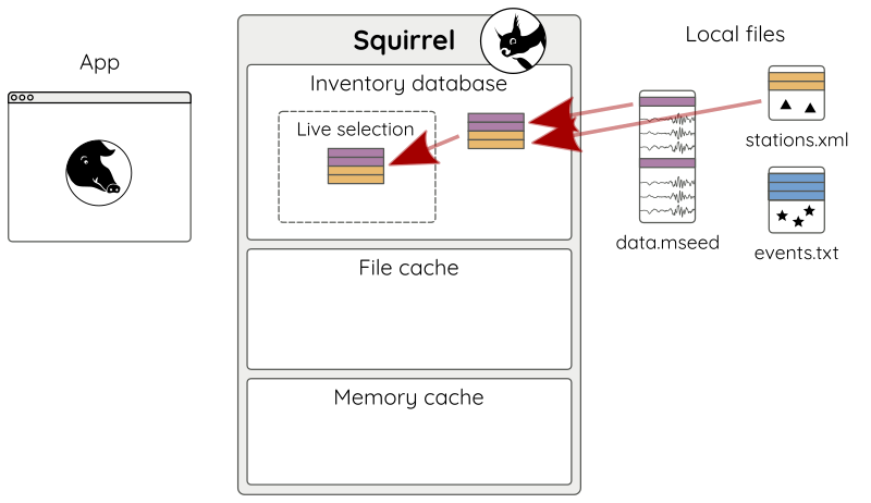
Figure 2: Adding local files.
Only a minimal excerpt from the file headers is included in the inventory database. This information includes time span, FDSN network/station/location/channel codes, and sampling rate of each entity. These entities are referred to as “nuts” in the Squirrel framework. A nut may represent a station or channel epoch, a snippet of waveform, or an instrument response epoch, among a few others. Also earthquake catalog events can be included. Nuts representing earthquake events only have the time span attribute set and their codes attribute is set to a catalog identifier. Bulk data associated with the Nut stays in the file until it is requested.
Content can be added (and removed) efficiently at run-time. For example to additionally add some hypocenters from an event catalog, we may use:
sq.add('events.txt')
Inventory information is updated as needed (Fig. 3).
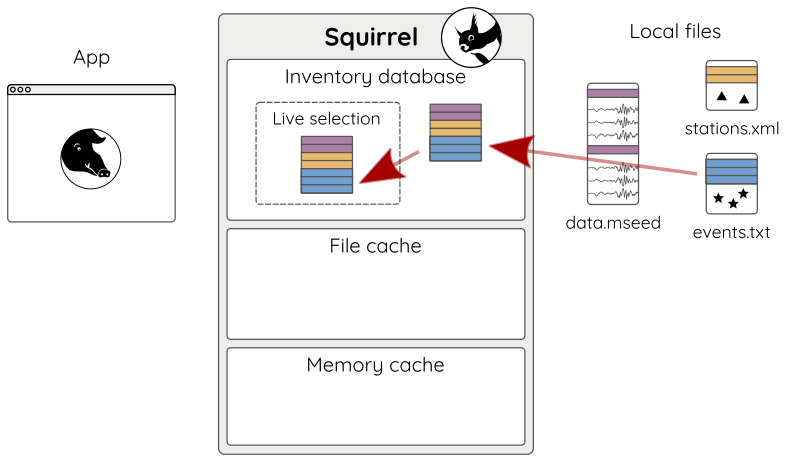
Figure 3: Adding another file - here an event catalog.
Content queries
Content of the live selection can be queried with the various getters
(.get_* methods) of the Squirrel object.
For example to get all stations as squirrel.Station objects, use:
stations = sq.get_stations()
Querying is performed on the index in the live selection. When there is a hit, associated bulk data is loaded from the respective file into a memory cache and a reference is returned to the application (Fig 4).
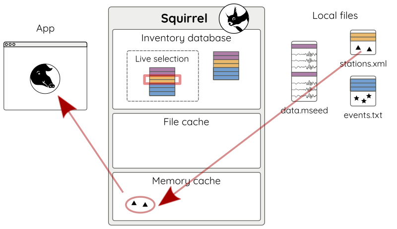
Figure 4: First query for content. Content is loaded into the memory cache and a reference is returned to the app.
It is possible to efficiently query by station/channel codes and time spans.
stations = sq.get_stations(codes='*.STA23.*.*')
In this case we have a cache hit and no data has to be loaded from file (Fig. 5).
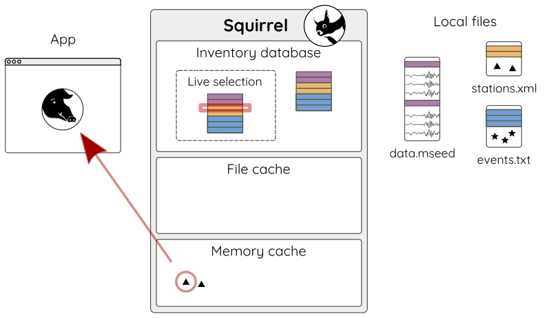
Figure 5: Subsequent query for content. As it is already loaded only a reference to the cached object is returned.
The getters provide an easy way to access associated data. For example, to get all channels of a given station, use:
channels = sq.get_channels(station)
Or to get an excerpt of the waveforms for some channel in a given time interval:
traces = sq.get_waveforms(channel, tmin=tmin, tmax=tmax)
Or to get the appropriate instrument response for a given waveform:
response = sq.get_response(trace)
The getters share a consistent interface where possible. Details are given in
the documentation of the Squirrel class in
the reference manual.
Content indexing details
Of course, it is also possible to selectively remove content from the Squirrel instance:
sq.remove('stations.xml')
When using remove(), only index
entries in the live selection are removed (Fig. 6).
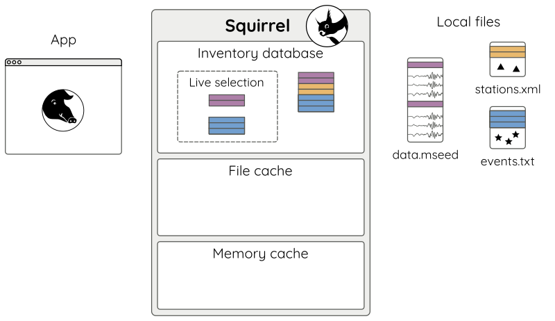
Figure 6: Removing stuff: sq.remove('stations.xml') - content from
stations.xml is now unavailable to the application.
When the application exits, its live selection vanishes (Fig 7).
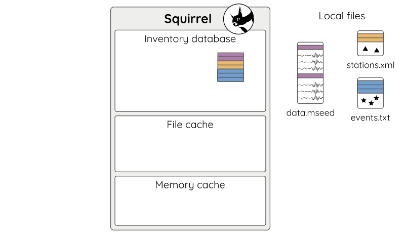
Figure 7: The application has quit. Index information is retained in the database.
When the application is restarted, it starts again with an empty live selection (Fig 8).
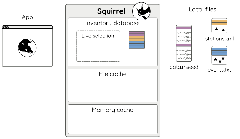
Figure 8: Application has been restarted.
But now, adding already known content is fast (Fig 9 a).
sq.add('data.mseed') # updates index as needed
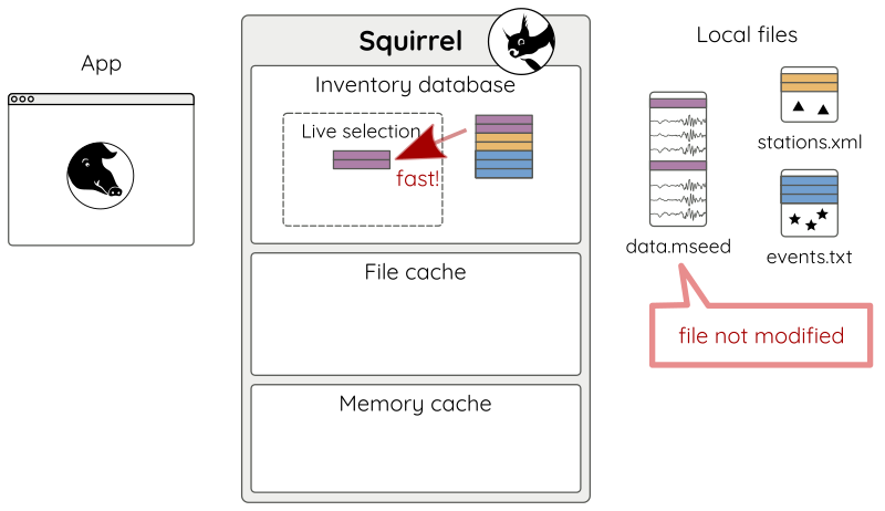
Figure 9 a: Adding unmodified files.
By default, the modification times of the files are checked to decide if re-indexing is needed (Fig 9 b).
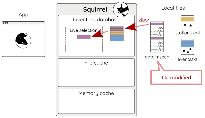
Figure 9 b: Adding modified files.
For an additional speedup, the modification time checks can be disabled (Fig 9 c):
sq.add('data.mseed', check=False) # only index if unknown
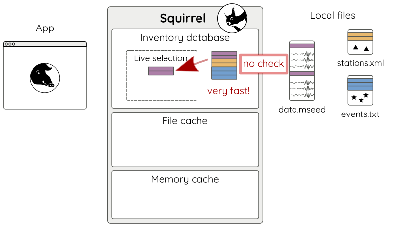
Figure 9 c: Adding files with check=False.
Modified files will still be recognized and handled appropriately, but only later, during content access queries.
Persistent selections
Let’s start another app and add some content.
# other app
sq = Squirrel()
sq.add('stations.xml')  # selection is private by default
Applications running in the same Squirrel environment share the database of indexed content but each application has its own live selection (Fig 10).
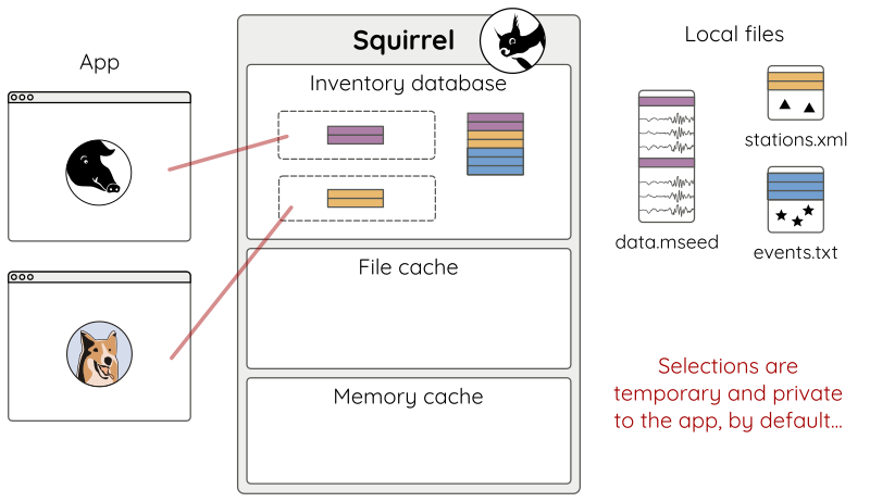
Figure 10: Multiple applications using the same Squirrel environment.
Selections can be made persistent and are shared among multiple applications using the same Squirrel environment (Fig 11):
# In one app:
sq = Squirrel(persistent='S1')  # use selection named "S1"
sq.add('data.mseed')

# In the other app:
sq = Squirrel(persistent='S1')
# No need to add('data.mseed') it is already there.
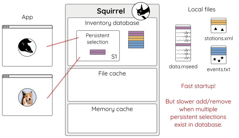
Figure 11: Multiple applications sharing a persistent selection.
Persistent selection are especially useful when dealing with huge datasets
because the run-time data selection does not have to be re-created at each
application startup. The speedup is huge, but the persistent selections also
add some bookkeeping overhead to the database, so don’t overuse them. Use
squirrel persistent to manage your persistent selections.
Online data access
A Squirrel instance can be made aware of
remote data sources. For example we could add the GE network from the GEOFON
FDSN web service as a data source (Fig 12):
sq.add_fdsn('geofon', query_args={'network': 'GE'})
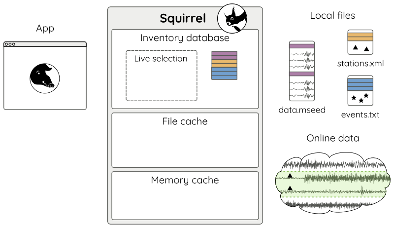
Figure 12: A remote data source.
Using add_fdsn() has no immediate
effect on what is available. We must first call
update() to refresh the local
inventory.
sq.update(tmin=tmin, tmax=tmax) # time span of interest (tmin, tmax)
This will get the channel metadata (Fig. 13).
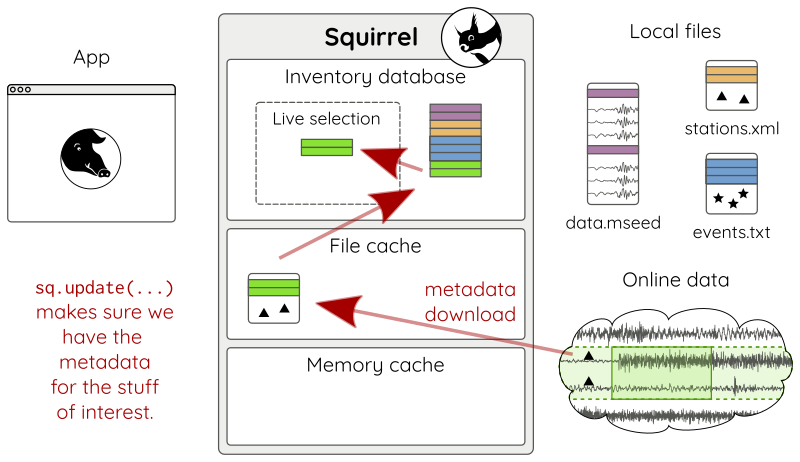
Figure 13: Metadata is downloaded and made available locally.
Metadata is cached locally so further calls to
update() won’t produce any queries to
the FDSN service. If needed, it is possible to set an expiration date on the
metadata from a specific FDSN site
(expires).
To enable downloads of selected waveforms it is required to set up so-called “waveform promises” for these
sq.update_waveform_promises(tmin=tmin, tmax=tmax, codes='GE.*.*.LHZ')
With update_waveform_promises()
promises are created, based on matching channels and time spans (Fig. 14).
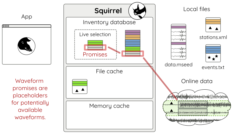
Figure 14: Waveform promises have been created with
update_waveform_promises().
Promises are resolved during queries like
get_waveforms():
sq.get_waveforms(tmin=tmin, tmax=tmax, codes='GE.STA23..LHZ')
If the query hits a promise (Fig 15 a), enough waveforms are downloaded in chunks of reasonable size (Fig 15 b), so that afterwards the waveform query can be normally resolved just like with local data (Fig 15 c).
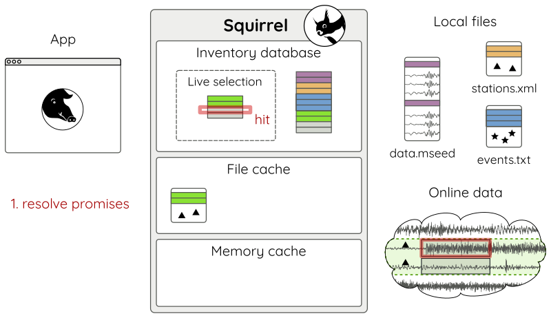
Figure 15 a: Resolving waveform promises - (1) query hit.
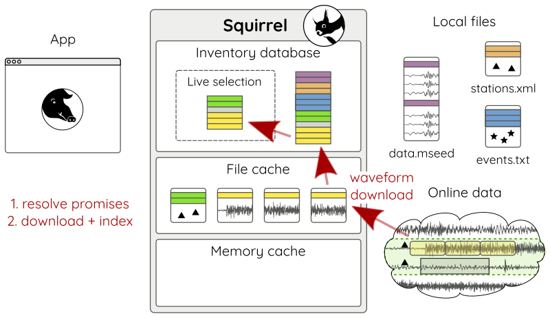
Figure 15 b: Resolving waveform promises - (2) download and index.
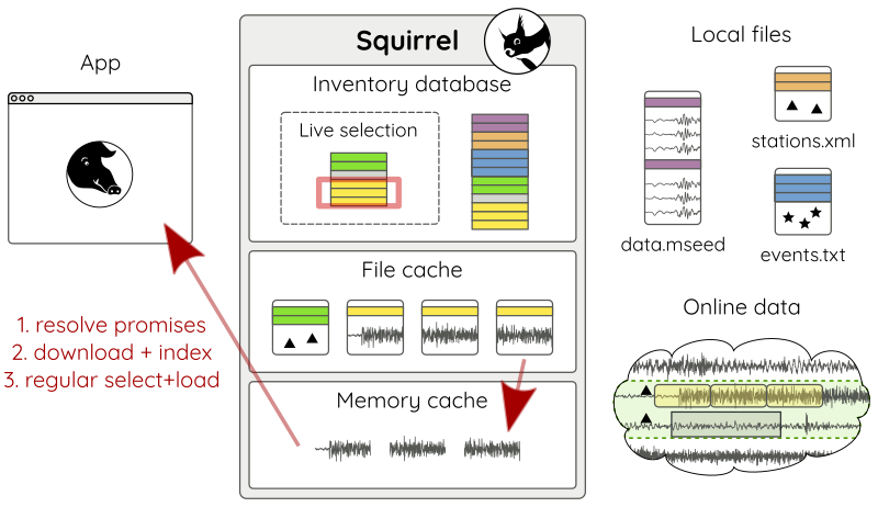
Figure 15 c: Resolving waveform promises - (3) select and load.
Set up like this, data can be downloaded just when needed and already downloaded data will be used together with local data and metadata through one unified interface.
Next steps
If you wish to use Squirrel in your own script, see Tutorial: writing a Squirrel based tool to calculate hourly RMS values. To learn more about data handling with the Squirrel in general, see Squirrel command line tool tutorial.