
Pseudo Dynamic Rupture - A stress-based self-similar finite source model
Introduction
Physics-based, dynamic rupture models, which rely on few parameters only, are needed for realistic forward modelling and to reduce the effort and non-uniqueness of the inversion. The PseudoDynamicRupture is a simplified, quasi-dynamic, semi-analytical rupture model suited for wavefield and static displacement simulation and earthquake source inversion. The rupture model builds on the class of self-similar crack models. On one hand it is approximative as it neglects inertia and so far the details of frictional effects and treats the rupture front growth in a simplified way. On the other hand, it is complete as the slip fulfils the boundary condition on the broken plane for every instantaneous rupture front geometry and applied stress.
Additional resources
The pseudo dynamic rupture model (introduction and practical examples)
Theoretical foundation
Note
Dahm, T., Heimann, S., Metz, M., Isken, M. P. (2021). A self-similar dynamic rupture model based on the simplified wave-rupture analogy. Geophysical Journal International. Volume 225, Issue 3, June 2021, Pages 1586–1604, https://doi.org/10.1093/gji/ggab045
Source implementation details
The implementation of the pseudo dynamic rupture model into the Pyrocko and Pyrocko-GF framework is based on [Dahm2021]. Essential building blocks are the class PseudoDynamicRupture and in the AbstractTractionField subclasses. Additionally the model is constrained by the subsurface underground model as provided by the metadata in the Pyrocko GF Store. See [Dahm2021] which describes the rupture source model in detail.

Flowchart illustrating the building blocks and architecture of the PseudoDynamicRupture in Pyrocko-GF.
Forward modelling a pseudo dynamic rupture
The PseudoDynamicRupture model is fully integrated into Pyrocko-GF. The model can be used to forward model synthetic waveforms, surface displacements and any quantity that is delivered by the store. Various utility functions are available to analyse and visualize parameters of the rupture model.
In this section we will show the parametrisation, introspection and resulting seismological forward calculations using the PseudoDynamicRupture.
Forward calculation of waveforms and static displacement
Parametrisation of the source model is straight forward, as for any other Pyrocko-GF source. In the below code example we parametrize a shallow bidirectional strike-slip source.
More details on dynamic and static Green’s function databases and other source models are laid out in section Pyrocko-GF - Geophysical forward modelling with pre-calculated Green’s functions.
Simple pseudo dynamic rupture forward model
We create a simple forward model and calculate waveforms for one seismic station (Target) at about 14 km distance - The tractions will be aligned to force the defined slip rake angle. The modeled waveform is displayed in the Snuffler application.
Important: the spatial sampling of the GF store used in the example must be dense enough to prevent aliasing artifacts.
Download gf_forward_pseudo_rupture_basic.py
import os.path as op
from pyrocko import gf

km = 1e3

# The store we are going extract data from:
store_id = 'iceland_reg_v2'

# First, download a Green's functions store. If you already have one that you
# would like to use, you can skip this step and point the *store_superdirs* to
# the containing directory.
if not op.exists(store_id):
    gf.ws.download_gf_store(site='pyrocko', store_id=store_id)

# We need a pyrocko.gf.Engine object which provides us with the traces
# extracted from the store. In this case we are going to use a local
# engine since we are going to query a local store.
engine = gf.LocalEngine(store_superdirs=['.'])

# The dynamic parameters used for discretization of the PseudoDynamicRupture
# are extracted from the store's config file.
store = engine.get_store(store_id)

# Let's define the source now with its extension, orientation etc.
rupture = gf.PseudoDynamicRupture(
    lat=0.,
    lon=0.,
    north_shift=2.*km,
    east_shift=2.*km,
    depth=3.*km,
    strike=43.,
    dip=89.,
    rake=88.,

    length=15*km,
    width=5*km,

    nx=10,
    ny=5,

    # Relative nucleation between -1. and 1.
    nucleation_x=-.6,
    nucleation_y=.3,
    slip=1.,
    anchor='top',

    # Threads used for modelling
    nthreads=1,

    # Force pure shear rupture
    pure_shear=True)

# Recalculate slip, so that the rupture's magnitude fits the given value
rupture.rescale_slip(magnitude=7.0, store=store)

# Create waveform target, where synthetic waveforms are calculated for
waveform_target = gf.Target(
    lat=0.,
    lon=0.,
    east_shift=10*km,
    north_shift=10.*km,
    interpolation='multilinear',
    store_id=store_id)

# Get synthetic waveforms and display them in snuffler
response = engine.process(rupture, waveform_target)
response.snuffle()
Traction and stress field parametrisation
The rupture plane can be exposed to different stress/traction field models which drive and interact with the rupture process.
A TractionField defines the absolute stress release on the fault plane:
An AbstractTractionField can modify an existing TractionField:
These fields can be used independently or be combined into a TractionComposition, where TractionField are stacked and AbstractTractionField are multiplied with the stack. See the reference and code for implementation details.
Pure tractions can be visualised using the utility function plot_tractions().
Plotting and rupture model insights
Convenience functions for plotting and introspection of the dynamic rupture model are offered by the pyrocko.plot.dynamic_rupture module.
Traction and rupture evolution
Initialize a simple dynamic rupture with uniform rake tractions and visualize the tractions and rupture propagation.
Download gf_forward_pseudo_rupture_basic_plot.py
import os.path as op
from pyrocko import gf
from pyrocko.plot.dynamic_rupture import RuptureView

km = 1e3

# The store we are going extract data from:
store_id = 'iceland_reg_v2'

# First, download a Green's functions store. If you already have one that you
# would like to use, you can skip this step and point the *store_superdirs* to
# the containing directory.
if not op.exists(store_id):
    gf.ws.download_gf_store(site='pyrocko', store_id=store_id)

# We need a pyrocko.gf.Engine object which provides us with the traces
# extracted from the store. In this case we are going to use a local
# engine since we are going to query a local store.
engine = gf.LocalEngine(store_superdirs=['.'])

# The dynamic parameters used for discretization of the PseudoDynamicRupture
# are extracted from the store's config file.
store = engine.get_store(store_id)

# Let's define the source now with its extension, orientation etc.
rupture = gf.PseudoDynamicRupture(
    # At lat 0. and lon 0. (default)
    north_shift=2.*km,
    east_shift=2.*km,
    depth=3.*km,
    strike=43.,
    dip=89.,
    rake=88.,

    length=15*km,
    width=5*km,

    nx=10,
    ny=5,

    # Relative nucleation between -1. and 1.
    nucleation_x=-.6,
    nucleation_y=.3,
    slip=1.,
    anchor='top',

    # Threads used for modelling
    nthreads=1,

    # Force pure shear rupture
    pure_shear=True)

# Recalculate slip, that rupture magnitude fits given magnitude
rupture.rescale_slip(magnitude=7.0, store=store)

plot = RuptureView(rupture, figsize=(8, 4))
plot.draw_patch_parameter('traction')
plot.draw_time_contour(store)
plot.draw_nucleation_point()
plot.save('dynamic_basic_tractions.png')
# Alternatively plot on screen
# plot.show_plot()
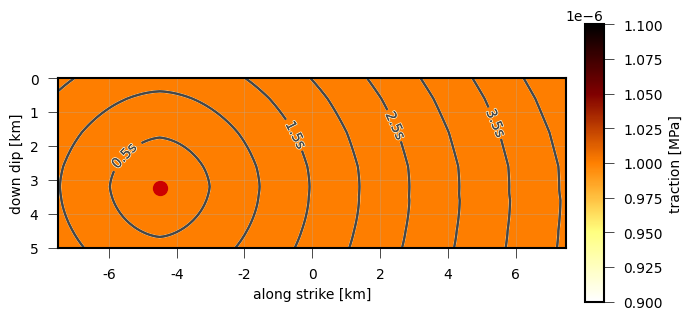
Absolute tractions of a simple dynamic source model with a uniform rake. Contour lines are isochrones of the rupture front.
Rupture propagation
We can investigate the rupture propagation speed  with
with draw_patch_parameter().
Rupture speed is proportional to the S-wave velocity in the Earth model and scaled with the attribute gamma.
# rupture is a PseudoDynamicRupture object
plot = RuptureView(rupture)

plot.draw_patch_parameter('vr')
plot.draw_time_contour(store)
plot.draw_nucleation_point()
plot.show_plot()
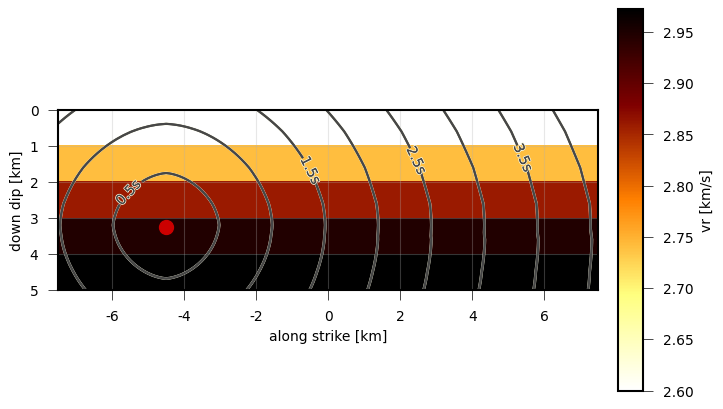
Rupture propagation speed of a simple dynamic source model. Contour lines are isochrones of the rupture front.
Slip distribution
Dislocations of the dynamic rupture source can be plotted with draw_dislocation():
# rupture is a PseudoDynamicRupture object
plot = RuptureView(rupture)

plot.draw_dislocation()
plot.draw_time_contour(store)
plot.draw_nucleation_point()
plot.show_plot()
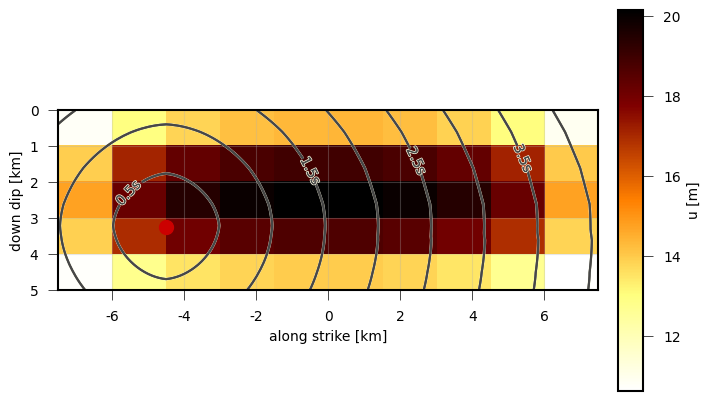
Absolute dislocation of a simple dynamic rupture source model with uniform rake tractions. Contour lines are isochrones of the rupture front.
Rupture evolution
We can animate the rupture evolution using the rupture_movie() function.
from pyrocko.plot.dynamic_rupture import rupture_movie

rupture_movie(
    rupture, store, 'dislocation',
    plot_type='view')
Combined complex traction fields
In this example we will combine different traction fields: DirectedTractions, FractalTractions and taper them using RectangularTaper.
After plotting the tractions and final dislocations, we will forward model the waveforms.
Download gf_forward_pseudo_rupture_complex.py
import os.path as op

from pyrocko import gf
from pyrocko.plot.dynamic_rupture import RuptureView

km = 1e3

# The store we are going extract data from:
store_id = 'iceland_reg_v2'

# First, download a Green's functions store. If you already have one that you
# would like to use, you can skip this step and point the *store_superdirs* to
# the containing directory.
if not op.exists(store_id):
    gf.ws.download_gf_store(site='pyrocko', store_id=store_id)

# We need a pyrocko.gf.Engine object which provides us with the traces
# extracted from the store. In this case we are going to use a local
# engine since we are going to query a local store.
engine = gf.LocalEngine(store_superdirs=['.'])

# The dynamic parameters used for discretization of the PseudoDynamicRupture
# are extracted from the store's config file.
store = engine.get_store(store_id)

# Let's define the source now with its extension, orientation etc.
rupture = gf.PseudoDynamicRupture(
    lat=0.,
    lon=0.,
    north_shift=2.*km,
    east_shift=2.*km,
    depth=3.*km,
    strike=43.,
    dip=89.,

    length=15*km,
    width=5*km,

    nx=10,
    ny=5,

    # Relative nucleation between -1. and 1.
    nucleation_x=-.6,
    nucleation_y=.3,

    # Relation between subsurface model s-wave velocity vs
    # and rupture velocity vr
    gamma=0.7,

    slip=1.,
    anchor='top',

    # Threads used for modelling
    nthreads=1,

    # Force pure shear rupture
    pure_shear=True,

    # Tractions are in [Pa]. However here we are using relative tractions,
    # Resulting waveforms will be scaled to the maximumslip [m]
    tractions=gf.tractions.TractionComposition(
        components=[
            gf.tractions.DirectedTractions(rake=56., traction=1.e6),
            gf.tractions.FractalTractions(rake=56., traction_max=.4e6),
            gf.tractions.RectangularTaper()
        ])
)

rupture.discretize_patches(store)

# Plot the absolute tractions from strike, dip, normal
plot = RuptureView(rupture, figsize=(8, 4))
plot.draw_patch_parameter('traction')
plot.draw_nucleation_point()
plot.save('dynamic_complex_tractions.png')

# Plot the modelled dislocations
plot = RuptureView(rupture, figsize=(8, 4))
plot.draw_dislocation()
# We can also define a time for the snapshot:
# plot.draw_dislocation(time=1.5)
plot.draw_time_contour(store)
plot.draw_nucleation_point()
plot.save('dynamic_complex_dislocations.png')

# Forward model waveforms for one station
engine = gf.LocalEngine(store_superdirs=['.'])
store = engine.get_store(store_id)

waveform_target = gf.Target(
    lat=0.,
    lon=0.,
    east_shift=10*km,
    north_shift=30.*km,
    interpolation='multilinear',
    store_id=store_id)

response = engine.process(rupture, waveform_target)
response.snuffle()
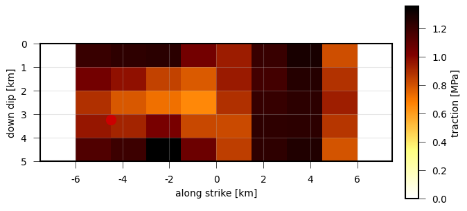
Absolute tractions of a complex dynamic rupture source model with uniform rake and superimposed random fractal perturbations.
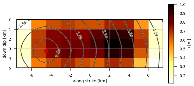
Absolute dislocation of a complex dynamic rupture source with uniform rake and superimposed random fractal perturbations. Contour lines are isochrones of the rupture front.
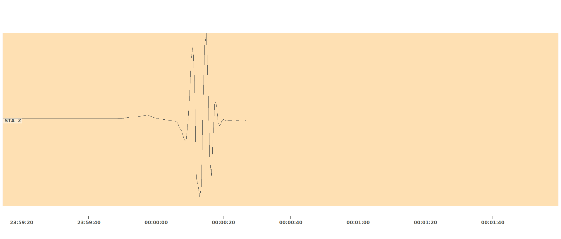
Synthetic waveforms generated by Pyrocko-GF from the pseudo dynamic rupture model at 31 km distance.
Moment rate function / source time function
With this example we demonstrate, how the moment rate  or source time function (STF) of a rupture can be simulated using the slip rate on each subfault
  , the average shear modulus
  and the subfault areas
  :
:

Use the method draw_source_dynamics():
plot = RuptureView(rupture)

# variable can be:
#    - 'stf', 'moment_rate':            moment rate function
#    - 'cumulative_moment', 'moment':   cumulative seismic moment function
# of the rupture
plot.draw_source_dynamics(variable='stf', store=store)
plot.show_plot()
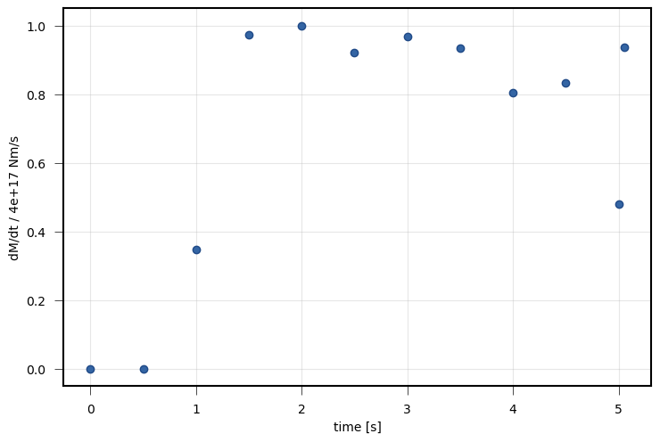
Source time function (moment rate function) of the complex dynamic rupture source model with uniform rake and superimposed random fractal perturbations.
Individual time-dependent subfault characteristics
Sometimes it might be also interesting to check the time-dependent behaviour of an individual subfault.
Use the method draw_patch_dynamics():
plot = RuptureView(rupture)

# nx and ny are the indices of the subfault along strike (nx) and down dip (ny)
# variable can be:
#    - 'dislocation':                   length of subfault dislocation vector [m]
#    - 'dislocation_<x, y, z>':         subfault dislocation vector component
#                                       in strike, updip or normal direction in [m]
#    - 'slip_rate':                     subfault slip rate in [m/s]
#    - 'moment_rate':                   subfault moment rate function
#    - 'cumulative_moment', 'moment':   subfault summed moment function
# of the rupture
plot.draw_patch_dynamics(variable='slip_rate', nx=6, ny=3, store=store)
plot.show_plot()
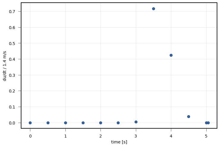
Slip rate function of a single subfault ( ) of the complex dynamic rupture source with uniform rake tractions and random fractal perturbations.
Radiated seismic energy
For rather complex ruptures also directivity effects in the waveforms are of interest. Using the function plot_directivity() allows to plot synthetic waveforms or its envelopes at a certain distance from the source in a circular plot. It provides an easy way of visual directivity effect imaging.
from pyrocko.plot.directivity import plot_directivity

# many more possible arguments are provided in the help of plot_directivity
resp = plot_directivity(
    engine,
    rupture,
    store_id,
    phases={
        'P': '{cake:p|cake:P}-10%',
        'S': '{cake:s|cake:S}+50'},

    # distance and azimuthal density of modelled waveforms
    distance=300*km,
    dazi=5.,

    # waveform settings
    component='R',
    quantity='displacement',
    envelope=True,

    plot_mt='full')
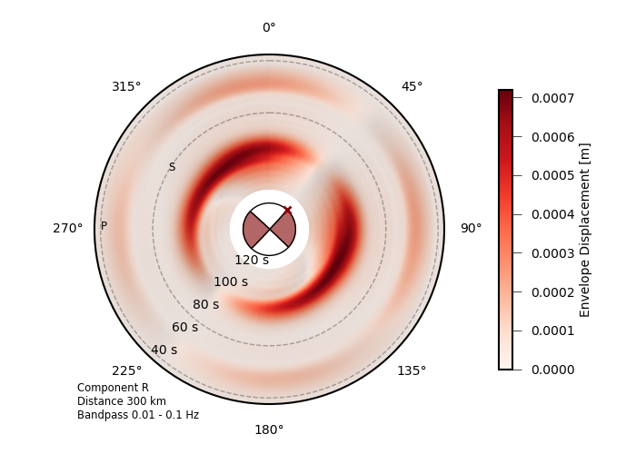
Directivity plot at 300 km distance for the complex dynamic rupture source with uniform rake tractions and random fractal perturbations.
References
Dahm, T., Heimann, S., Metz, M., Isken, M. P. (2021). A self-similar dynamic rupture model based on the simplified wave-rupture analogy. Geophysical Journal International. Volume 225, Issue 3, June 2021, Pages 1586–1604, https://doi.org/10.1093/gji/ggab045