
How to setup a Custom Greens Function Store
This section covers how to generate a custom Greens Function store for seismic data at a location of choice. First a new model project has to be created to generate the configuration file. As we have no specific event in mind we skip the catalog search by not specifying the date.:
beat init Cascadia --datatypes='seismic' --mode='geometry' --use_custom
Note
To use the default ak135 earth-model in combination with crust2 one needs to execute above command without the ‘–use_custom’ flag.
This will create a beat project folder named ‘Cascadia’ and a configuration file ‘config_geometry.yaml’. In this configuration file we may now edit the reference location and the velocity model to the specific model we received from a colleague or found in the literature.:
cd Cascadia
vi config_geometry.yaml
This will open the configuration file in the vi editor. In lines 4-6 we find the reference event:
event: !pf.Event
  lat: 0.0
  lon: 0.0
In lines 160-165 we find the reference location:
reference_location: !beat.heart.ReferenceLocation
  lat: 10.0
  lon: 10.0
  elevation: 0.0
  depth: 0.0
  station: Store_Name
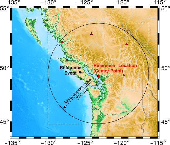
The distance between these two locations determines the center point of the grid of Greens Functions that we want to calculate. The following image (contributed by So-Young Baag) sketches the geometry of an example setup.
For our example we set the reference location close to Vancouver, Canada as we want to study the Cascadia subduction zone. We ignore the ‘elevation’ and ‘depth’ attributes but we set the ‘station’ attribute, which determines the prefix of the name of the Greens Function store.
reference_location: !beat.heart.ReferenceLocation
  lat: 49.28098
  lon: -123.12244
  elevation: 0.0
  depth: 0.0
  station: Vancouver
The events we want to study are going to be around Vancouver island, and we set the reference event coordinates accordingly:
event: !pf.Event
  lat: 49.608839
  lon: -125.647683
So far we determined the general location of the store, but now we need to specify the spatial dimensions of the grid. In lines 154-158 we find the respective parameters:
source_depth_min: 0.0
source_depth_max: 10.0
source_depth_spacing: 1.0
source_distance_radius: 20.0
source_distance_spacing: 1.0
We are going to have stations in a distance of 500km and the events we are going to study are going to be located in a depth range of 5-40km depth so we update these values accordingly.:
source_depth_min: 5.0
source_depth_max: 40.0
source_depth_spacing: 1.0
source_distance_radius: 500.0
source_distance_spacing: 1.0
To decide on the resolution of the grid and the sample_rate (line 167) depends on the use-case and aim of the study. A description of the corner points to have in mind is here For example for a regional Full Moment Tensor inversion we want to optimize data up to 0.2 Hz. So a source grid of 1. km step size and 1. Hz ‘sample_rate’ seems a safe way to go. As we are in a regional setup we use QSEIS for the calculation of the Greens Functions, which we have to specify in line 166.:
code: qseis
In the lines 144-153 is the velocity model defined for which the Greens Functions are going to be calculated.:
custom_velocity_model: |2
      0.             5.8            3.46           2.6         1264.           600.
     20.             5.8            3.46           2.6         1264.           600.
     20.             6.5            3.85           2.9         1283.           600.
     35.             6.5            3.85           2.9         1283.           600.
  mantle
     35.             8.04           4.48           3.58        1449.           600.
     77.5            8.045          4.49           3.5         1445.           600.
     77.5            8.045          4.49           3.5          180.6           75.
    100.             8.048          4.495          3.461        180.3           75.
The columns are ‘depth’, ‘p-wave velocity’, ‘s-wave velocity’, ‘density’, ‘Qp’, ‘Qs’. Here the values may be changed to a custom velociy. For example if we want to add another layer (from 20-25 km depth) between 20 and 35 km depth we would write:
custom_velocity_model: |2
      0.             5.8            3.46           2.6         1264.           600.
     20.             5.8            3.46           2.6         1264.           600.
     20.             6.1            3.54           2.7         1280.           600.
     25.             6.1            3.54           2.7         1280.           600.
     25.             6.5            3.85           2.9         1283.           600.
     35.             6.5            3.85           2.9         1283.           600.
  mantle
     35.             8.04           4.48           3.58        1449.           600.
     77.5            8.045          4.49           3.5         1445.           600.
     77.5            8.045          4.49           3.5          180.6           75.
    100.             8.048          4.495          3.461        180.3           75.
Below the specified depth it is going to be combined with the earth-model specified in line 141.
Note
In case the standard earth-model should be used rather than a custom model the ‘custom_velocity_model’ attribute may be deleted. For the shallow crust one may decide to use the implemented crust2 model and to remove (potential) water layers. Lines 141-143:
earth_model_name: ak135-f-average.m
use_crust2: false
replace_water: false
Then, we have to specify under line 135 ‘store_superdir’ the path to the directory where to save the GreensFunction store on disk. One should have in mind that for large grids with high sample-rate the stores might become several GigaBytes in size and may calculate a very long time!
Lastly, we start the store calculation with:
beat build_gfs Cascadia --execute --datatypes='seismic'