
How to setup a Finite Fault Inference
With the finite fault inference (ffi) mode in beat a pre-defined RectangularSource (reference fault) is discretized into sub-patches. Each of these sub-patches may have up to 4 parameters to be optimized for. In the static case (geodetic data) these are two slip-parameters perpendicular and parallel to the rake direction of the reference fault. In the kinematic case there is the temporal evolution of the rupture considered as well. So there are additional parameters: (1) the rupture nucleation point from which the rupture originates and propagates across the fault following the eikonal equation, (2) the slip-duration and the rupture velocity across each sub-patch. Each sub-patch is considered to be active only once. Optimizing for the rupture nucleation point makes the problem non-linear.
The finite fault inference in beat is considered to be a follow-up step of the geometry estimation for a RectangularSource. Which is why first, a new project directory to solve for the geometry of a RectangularSource has to be created. If the reader has setup such a problem already and finished the sampling for a the geometry the next command can be skipped.:
beat init FFIproject <date> --datatypes='seismic' --source_types='RectangularSource' --n_sources=1
If an estimation for the geometry of another source has been done or setup (e.g. MTSource), one can clone this project folder and replace the source object. This saves time for specification of the inputs. How to setup the configurations for a “geometry” estimation is discussed here exemplary on a MomentTensor for regional seismic data. The “source_types” argument will replace any existing source with the specified sources for the new project. With the next project we replace the old source with a RectangularSource.:
beat clone MTproject FFIproject --datatypes='seismic' --source_types='RectangularSource' --copy_data
Now the Green’s Functions store(s) have to be calculated for the “geometry” problem if not done so yet. Instructions on this and what to keep in mind are given here. For illustration, the user might have done a MomentTensor estimation already on teleseismic data using Green’s Functions depth and distance sampling of 1km with 1Hz sampling. This may be accurate enough for this type of problem, however for a finite fault inference the aim is to resolve details of the rupture propagation and the slip distribution. So the setup parameters of the “geometry” Green’s Functions would need to be changed to higher resolution. A depth and distance sampling of 250m and 4Hz sample rate might be precise enough, if waveforms up to 1Hz are to be used in the sampling. Of course, these parameters depend on the problem setup and have to be adjusted individually for each problem!
If the Green’s Functions for the “geometry” have been calculated previously with sufficient accuracy one can continue initialising the configuration file for the finite fault inference.:
beat init FFIproject --mode='ffi' --datatypes='seismic'
This will load the parameters from the “geometry” problem and import them to the “ffi” setup. The configuration file for the “ffi” mode is called “config_ffi.yaml” and should be in the same directory as the “config_geometry.yaml”. The parameters that are different in the “ffi” mode are under the “seismic_config.gf_config” of the mentioned configuration file.:
gf_config: !beat.SeismicLinearGFConfig
  store_superdir: ./
  reference_model_idx: 0
  n_variations: [0, 1]
  earth_model_name: local
  nworkers: 3
  reference_sources:
  - !beat.sources.RectangularSource
    lat: 50.410785
    lon: -150.305465
    elevation: 0.0
    depth: 1000.0
    time: 1970-01-01 00:00:00
    stf: !pf.HalfSinusoidSTF
      duration: 15.0
      anchor: 0.0
    stf_mode: post
    magnitude: 6.0
    strike: 90.0
    dip: 67.5
    rake: 0.0
    width: 5000.0
    length: 10000.0
    slip: 4.05
    opening: 0.0
  patch_width: 2.5
  patch_length: 2.5
  extension_width: 0.0
  extension_length: 0.1
  sample_rate: 10.0
  reference_location: !beat.heart.ReferenceLocation
    lat: 50.0
    lon: -100.0
    elevation: 0.0
    depth: 0.0
    station: Waskahigan_broadband2
  duration_sampling: 1.0
  starttime_sampling: 1.0
In the next step again Green’s Functions have to be calculated. What? Again? That’s right! This time the geometry of the source needs to be specified. This is defined under the “reference_sources” attribute (see above). The distance units are [m], the angles [deg] and the slip [m]. If the sampling for these “geometry” parameters has been completed, the maximum likelihood result may be imported with.:
beat import FFIproject --results=/path_to_geometry_project --datatypes='seismic' --mode='geometry'
If not, the parameters would need to be adjusted manually based on a-priori information from structural geology, literature or … Additionally, the discretization of the subpatches along this reference fault has to be set. The parameters “patch_width” and “patch_length” [km] determine these. So far only square patches are supported. “extension_width” and “extension_length” determine by how much the reference fault is extended in EACH direction. If this would result in a fault that cuts the surface the intersection with the surface at zero depth is used. Example: 0.1 means that the fault is extended by 10% of its with/length value in each direction and 0. means no extension.
The “store_superdir” to the “geometry” Green’s Functions needs to be correct and the “sample_rate” needs to be set likely higher than from the “geometry” setup. The last two parameters are “duration_sampling” and “starttime_sampling” for the sampling of the source-time-function (STF) for each patch. For efficiency during sampling the STF is convolved for each source patch with the synthetic seismogram. The upper and lower bound for the STF duration and the STF (rupture) starttimes are determined by the problem parameters in the “priors” under “problem_config”.:
priors:
  durations: !beat.heart.Parameter
    name: durations
    form: Uniform
    lower: [0.5]
    upper: [15.5]
    testvalue: [10.0]
  nucleation_dip: !beat.heart.Parameter
    name: nucleation_dip
    form: Uniform
    lower: [0.0]
    upper: [7.0]
    testvalue: [3.5]
  nucleation_strike: !beat.heart.Parameter
    name: nucleation_strike
    form: Uniform
    lower: [0.0]
    upper: [10.0]
    testvalue: [5.0]
  uparr: !beat.heart.Parameter
    name: uparr
    form: Uniform
    lower: [-0.3]
    upper: [6.0]
    testvalue: [2.85]
  uperp: !beat.heart.Parameter
    name: uperp
    form: Uniform
    lower: [-0.3]
    upper: [4.0]
    testvalue: [1.85]
  velocities: !beat.heart.Parameter
    name: velocities
    form: Uniform
    lower: [0.5]
    upper: [4.2]
    testvalue: [2.35]
For this example the synthetic seismograms ranging from an STF with a slip-duration of 0.5s up to 15.5s with a sampling of 1s would be calculated (0.5, 1.5, 2.5). The sampling has to be consistent with the start and end durations. For example a duration lower: 0.5, duration upper: 3., with a sampling of 0.4 would result in an error as the sampling steps would be: 0.5, 0.9, 1.3, 1.7, 2.1, 2.5, 2.9 but 3. is not included. The “velocities” parameter is referring to the rupture velocity, which is often considered to be propagating with S-wave velocity. Depending on the velocity model that has been used during the setup of the “geometry” Green’s Functions these parameter bounds may be adjusted.
With the following command the reference fault is set up and discretized into patches.:
beat build_gfs FFIproject --mode='ffi' --datatypes='seismic'
The output might look like this:
ffi          - INFO     Discretizing seismic source(s)
ffi          - INFO     uparr slip component
sources      - INFO     Fault extended to length=12500.000000, width=5000.000000!
ffi          - INFO     Extended fault(s):
 --- !beat.sources.RectangularSource
lat: 50.410785
lon: -150.305465
elevation: 0.0
depth: 1000.0
time: 1970-01-01 00:00:00
stf: !pf.HalfSinusoidSTF
  duration: 15.0
  anchor: 0.0
stf_mode: post
magnitude: 6.0
strike: 90.0
dip: 67.5
rake: 0.0
width: 5000.0
length: 12500.0
slip: 1.0
opening: 0.0

ffi          - INFO     uperp slip component
sources      - INFO     Fault extended to length=12500.000000, width=5000.000000!
ffi          - INFO     Extended fault(s):
 --- !beat.sources.RectangularSource
lat: 50.410785
lon: -150.305465
elevation: 0.0
depth: 1000.0
time: 1970-01-01 00:00:00
stf: !pf.HalfSinusoidSTF
  duration: 15.0
  anchor: 0.0
stf_mode: post
magnitude: 6.0
strike: 90.0
dip: 67.5
rake: -90.0
width: 5000.0
length: 12500.0
slip: 1.0
opening: 0.0

beat         - INFO     Storing discretized fault geometry to: /home/vasyurhm/BEATS/Waskahigan2Rect/ffi/linear_gfs/fault_geometry.pkl
beat         - INFO     Updating problem_config:
beat         - INFO
Complex Fault Geometry
number of subfaults: 1
number of patches: 10
This shows the new parameters of the extended reference source. The “width” and “length” are rounded to full multiples of the “patch_length” and “patch_width” parameters. Also we see here the rake directions of the slip parallel and slip perpendicular directions. The hypocentral location bounds have been adjusted to be within the bounds of the extended fault dimensions! To allow for potential rupture nucleation all along the reference fault in the example, the priors of “nucleation_strike” and “nucleation_dip” were set to be between (0, 12.5)[km] and (0,5)[km], respectively! Of course, the bounds may be set manually to custom values within the fault dimensions!
Finally, we need to pay attention to the “waveforms” under “seismic_config”.:
waveforms:
- !beat.WaveformFitConfig
  include: true
  name: any_P
  channels: [Z]
  filterer:
  - !beat.heart.Filter
    lower_corner: 0.001
    upper_corner: 4.0
    order: 4
  distances: [0.0, 5.0]
  interpolation: multilinear
  arrival_taper: !beat.heart.ArrivalTaper
    a: -15.0
    b: -10.0
    c: 30.0
    d: 40.0
“Name” specifies the seismic phase; “channels” the component of the observations to include, “filterer” the bandpass filter the synthetics are filtered to; “distances” the receiver-source interval of receivers to include; and the “arrival_taper” the part of the synthetics with respect to the theoretical arrival time (from ray-tracing).
Once satisfied with the set-up the “nworkers” parameter in “config_ffi.yaml” may be set to make use of parallel calculation of the Green’s Functions. Depending on the specifications the amount of Green’s Functions to be calculated may-be significant. The resulting matrix will be of size: number_receivers * number_patches * number_durations * number_starttimes * number_trace_samples * float64 (8bytes).
The calculation of the Green’s Functions, which may take some hours (depending on the setup and computer hardware) may be started with:
beat build_gfs FFIproject --mode='ffi' --datatypes='seismic' --execute
For visual inspection of the resulting seismic traces in the “snuffler” waveform browser:
beat check FFIproject --what='library' --datatypes='seismic' --mode='ffi'
This will load the seismic traces for the first receiver, for all patches, durations, starttimes.
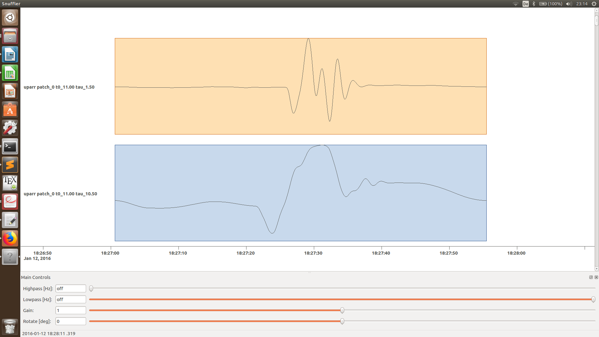
Here we see the slip parallel traces for patch 0, starttime of 11s (after the hypocentral source time) and slip durations(tau) of 1.5 and 10.5[s].