
Forward modeling synthetic seismograms and displacements
Calculate synthetic seismograms from a local GF store
It is assumed that a Store with store ID crust2_dd has been downloaded in advance. A list of currently available stores can be found at https://greens-mill.pyrocko.org as well as how to download such stores.
Further API documentation for the utilized objects can be found at Target, LocalEngine and DCSource.
Download gf_forward_example1.py
import os

from pyrocko.gf import LocalEngine, Target, DCSource, ws
from pyrocko import trace
from pyrocko.gui.snuffler.marker import PhaseMarker

# The store we are going extract data from:
store_id = 'iceland_reg_v2'

# First, download a Greens Functions store. If you already have one that you
# would like to use, you can skip this step and point the *store_superdirs* in
# the next step to that directory.

if not os.path.exists(store_id):
    ws.download_gf_store(site='pyrocko', store_id=store_id)

# We need a pyrocko.gf.Engine object which provides us with the traces
# extracted from the store. In this case we are going to use a local
# engine since we are going to query a local store.
engine = LocalEngine(store_superdirs=['.'])

# Define a list of pyrocko.gf.Target objects, representing the recording
# devices. In this case one station with a three component sensor will
# serve fine for demonstation.
channel_codes = 'ENZ'
targets = [
    Target(
        lat=10.,
        lon=10.,
        store_id=store_id,
        codes=('', 'STA', '', channel_code))
    for channel_code in channel_codes]

# Let's use a double couple source representation.
source_dc = DCSource(
    lat=11.,
    lon=11.,
    depth=10000.,
    strike=20.,
    dip=40.,
    rake=60.,
    magnitude=4.)

# Processing that data will return a pyrocko.gf.Reponse object.
response = engine.process(source_dc, targets)

# This will return a list of the requested traces:
synthetic_traces = response.pyrocko_traces()

# In addition to that it is also possible to extract interpolated travel times
# of phases which have been defined in the store's config file.
store = engine.get_store(store_id)

markers = []
for t in targets:
    dist = t.distance_to(source_dc)
    depth = source_dc.depth
    arrival_time = store.t('begin', (depth, dist))
    m = PhaseMarker(tmin=arrival_time,
                    tmax=arrival_time,
                    phasename='P',
                    nslc_ids=(t.codes,))
    markers.append(m)

# Finally, let's scrutinize these traces.
trace.snuffle(synthetic_traces, markers=markers)
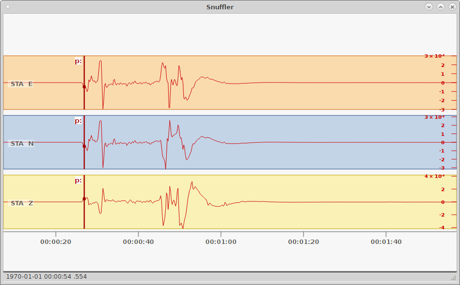
Synthetic seismograms calculated through pyrocko.gf displayed in Snuffler - seismogram browser and workbench. The three traces show the east, north and vertical synthetical displacement stimulated by a double-couple source at 155 km distance.
Calculate synthetic seismograms using the Pseudo Dynamic Rupture
Download gf_forward_pseudo_rupture_waveforms.py
import os.path as op

from pyrocko import gf

km = 1e3

# The store we are going extract data from:
store_id = 'crust2_mf'

# First, download a Greens Functions store. If you already have one that you
# would like to use, you can skip this step and point the *store_superdirs* in
# the next step to that directory.
if not op.exists(store_id):
    gf.ws.download_gf_store(site='pyrocko', store_id=store_id)

# We need a pyrocko.gf.Engine object which provides us with the traces
# extracted from the store. In this case we are going to use a local
# engine since we are going to query a local store.
engine = gf.LocalEngine(store_superdirs=['.'])

# The dynamic parameter used for discretization of the PseudoDynamicRupture are
# extracted from the stores config file.
store = engine.get_store(store_id)

# Let's define the source now with its extension, orientation etc.
dyn_rupture = gf.PseudoDynamicRupture(
    # At lat 0. and lon 0. (default)
    north_shift=2.*km,
    east_shift=2.*km,
    depth=3.*km,
    strike=43.,
    dip=89.,
    rake=88.,

    length=26.*km,
    width=12.*km,

    nx=10,
    ny=5,

    # Relative nucleation between -1. and 1.
    nucleation_x=-.6,
    nucleation_y=.3,
    slip=1.,
    anchor='top',

    # Threads used for modelling
    nthreads=1,

    # Force pure shear rupture
    pure_shear=True)

# Recalculate slip, that rupture magnitude fits given magnitude
dyn_rupture.rescale_slip(magnitude=7.0, store=store)

# Model waveforms for a single station target
waveform_target = gf.Target(
    lat=0.,
    lon=0.,
    east_shift=10.*km,
    north_shift=10.*km,
    store_id=store_id)

result = engine.process(dyn_rupture, waveform_target)
result.snuffle()
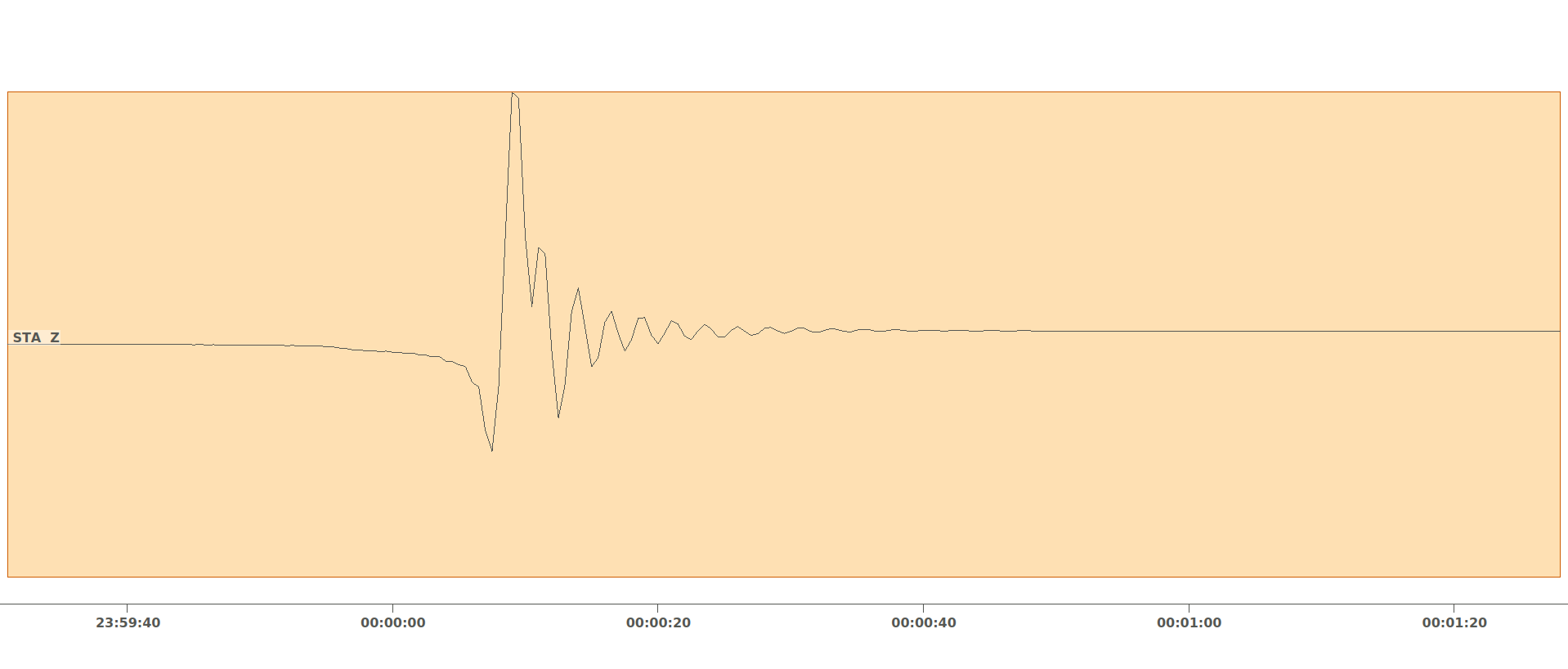
Synthetic seismogram calculated through pyrocko.gf using the
PseudoDynamicRupture.
Calculate Coulomb Failure Stress (CFS) changes using the Pseudo Dynamic Rupture
Download gf_forward_pseudo_rupture_cfs.py
'''
Coulomb Failure Stress (CFS) change calculation from pseudo-dynamic rupture.
'''
import os.path as op
import numpy as num

import matplotlib.pyplot as plt
import matplotlib.colors as colors

from pyrocko import gf, orthodrome as pod
from pyrocko.plot import mpl_init, mpl_papersize

# The store we are going extract data from:
store_id = 'gf_abruzzo_nearfield_vmod_Ameri'

# First, download a Greens Functions store. If you already have one that you
# would like to use, you can skip this step and point the *store_superdirs* in
# the next step to that directory.
if not op.exists(store_id):
    gf.ws.download_gf_store(site='pyrocko', store_id=store_id)

# We need a pyrocko.gf.Engine object which provides us with the traces
# extracted from the store. In this case we are going to use a local
# engine since we are going to query a local store.
engine = gf.LocalEngine(store_superdirs=['.'])

# The dynamic parameter used for discretization of the PseudoDynamicRupture are
# extracted from the stores config file.
store = engine.get_store(store_id)

# Let's define the source now with its extension, orientation etc.
source = gf.PseudoDynamicRupture(
    lat=37.718, lon=37.487, depth=5.3e3,
    length=213.8e3, width=21.3e3,
    strike=57.,
    dip=82.,
    rake=28.,
    slip=4.03,
    anchor='top',
    nx=6,
    ny=4,
    pure_shear=True,
    smooth_rupture=True)

# Calculate the subfault specific parameters
source.discretize_patches(store)

# Let's now define the target source now with its extension, orientation etc.
target = gf.PseudoDynamicRupture(
    lat=37.992, lon=37.262, depth=4.7e3,
    length=92.9e3, width=17.2e3,
    strike=-92.,
    dip=73.,
    rake=-8.,
    slip=7.07,
    # nucleation_x=-1.,
    # nucleation_y=0.,
    anchor='top',
    nx=6,
    ny=4,
    pure_shear=True,
    smooth_rupture=True)

# Define the receiver point locations, where the CFS will be calculated - here
# as a grid of (northing, easting, depth)
nnorths = 100
neasts = 100
norths = num.linspace(-200., 200., nnorths) * 1e3
easts = num.linspace(-200., 200., neasts) * 1e3
depth_target = 10e3

receiver_points = num.zeros((nnorths * neasts, 3))
receiver_points[:, 0] = num.repeat(norths, neasts)
receiver_points[:, 1] = num.tile(easts, nnorths)
receiver_points[:, 2] = num.ones(nnorths * neasts) * depth_target

# Calculate the Coulomb Failure Stress change (CFS) for the given target plane
strike_target = target.strike
dip_target = target.dip
rake_target = target.rake

cfs = source.get_coulomb_failure_stress(
    receiver_points, friction=0.6, pressure=0.,
    strike=strike_target, dip=dip_target, rake=rake_target, nthreads=2)

# Plot the results as a map
mpl_init(fontsize=12.)
fig, axes = plt.subplots(figsize=mpl_papersize('a5'))

# Plot of the Coulomb Failure Stress changes
mesh = axes.pcolormesh(
    easts / 1e3, norths / 1e3,
    cfs.reshape(neasts, nnorths) / 1e6,
    cmap='RdBu_r',
    shading='gouraud',
    norm=colors.SymLogNorm(
        linthresh=0.03, linscale=0.03, vmin=-1., vmax=1.))

# Plot the source plane as grey shaded area
fn, fe = source.outline(cs='xy').T
axes.fill(
    fe / 1e3, fn / 1e3,
    edgecolor=(0., 0., 0.),
    facecolor='grey',
    alpha=0.7)
axes.plot(fe[0:2] / 1e3, fn[0:2] / 1e3, 'k', linewidth=1.3)

# Plot the target plane as grey shaded area
north_shift, east_shift = pod.latlon_to_ne(
    source.lat, source.lon,
    target.lat, target.lon)
fn, fe = target.outline(cs='xy').T
fn += north_shift
fe += east_shift
axes.fill(
    fe / 1e3, fn / 1e3,
    edgecolor=(0., 0., 0.),
    facecolor='grey',
    alpha=0.7)
axes.plot(fe[0:2] / 1e3, fn[0:2] / 1e3, 'k', linewidth=1.3)

# Plot labeling
axes.set_xlabel('East shift [km]')
axes.set_ylabel('North shift [km]')
axes.set_title(
    f'Target plane: strike {strike_target:.0f}$^\\circ$, ' +
    f'dip {dip_target:.0f}$^\\circ$, ' +
    f'rake {rake_target:.0f}$^\\circ$, depth {depth_target/1e3:.0f} km')

cbar = fig.colorbar(mesh, ax=axes)
cbar.set_label(r'$\Delta$ CFS [MPa]')
cbar_ticks = [-1., -0.5, -0.25, -0.1, 0., 0.1, 0.25, 0.5, 1.]
cbar.set_ticks(cbar_ticks)
cbar.set_ticklabels([f'{tick:.2f}' for tick in cbar_ticks])

fig.savefig('gf_forward_pseudo_rupture_cfs.png')

plt.show()
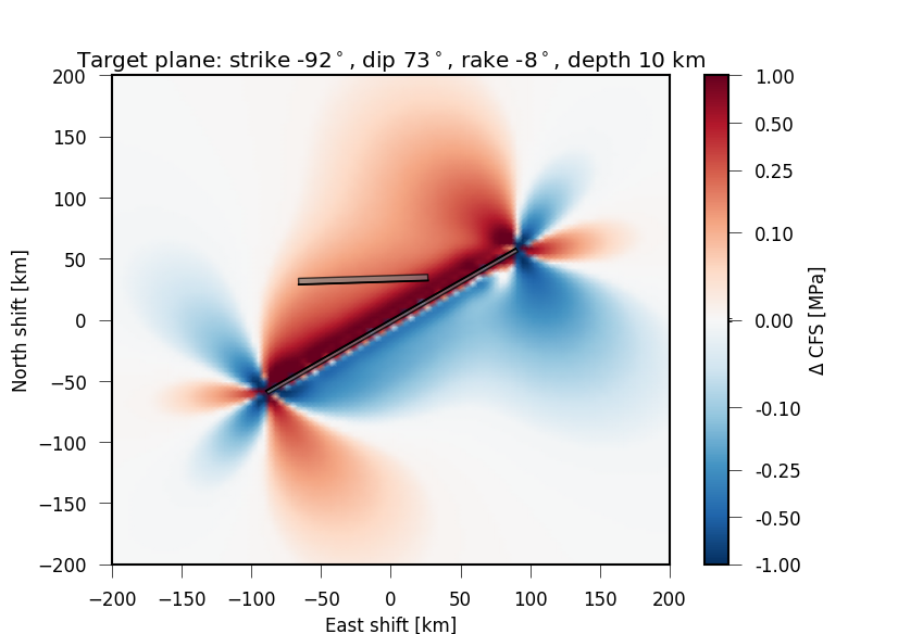
Coulomb Failure Stress change calculated through pyrocko.gf using
the PseudoDynamicRupture.
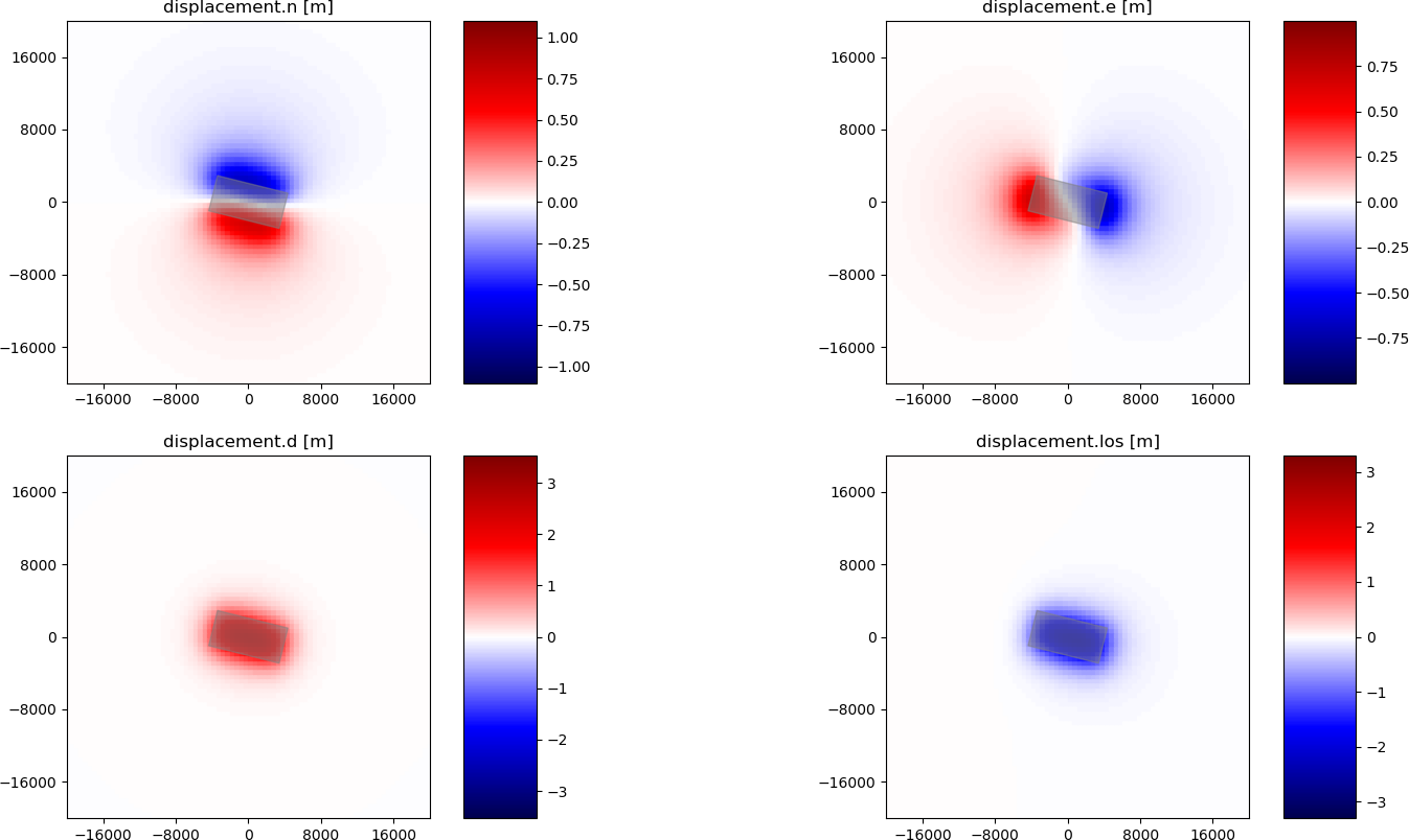
Calculate spatial surface displacement from a local GF store
Shear dislocation - Earthquake
In this example we create a RectangularSource and compute the spatial static displacement invoked by that rupture.
We will utilize LocalEngine, StaticTarget and SatelliteTarget.
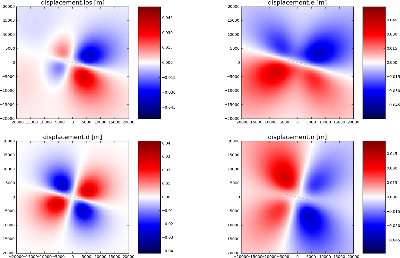
Synthetic surface displacement from a vertical strike-slip fault, with a N104W azimuth, in the Line-of-sight (LOS), east, north and vertical directions. LOS as for Envisat satellite (Look Angle: 23., Heading:-76). Positive motion toward the satellite.
Download gf_forward_example2.py
import os.path
from pyrocko import gf
import numpy as num

# Download a Greens Functions store, programmatically.
store_id = 'gf_abruzzo_nearfield_vmod_Ameri'
if not os.path.exists(store_id):
    gf.ws.download_gf_store(site='pyrocko', store_id=store_id)

# Setup the LocalEngine and point it to the fomosto store you just downloaded.
# *store_superdirs* is a list of directories where to look for GF Stores.
engine = gf.LocalEngine(store_superdirs=['.'])

# We define an extended source, in this case a rectangular geometry
# Centroid UTM position is defined relatively to geographical lat, lon position
# Purely lef-lateral strike-slip fault with an N104W azimuth.

km = 1e3  # for convenience

rect_source = gf.RectangularSource(
    lat=0., lon=0.,
    north_shift=0., east_shift=0., depth=6.5*km,
    width=5*km, length=8*km,
    dip=90., rake=0., strike=104.,
    slip=1.)

# We will define a grid of targets
# number in east and north directions, and total
ngrid = 80

# extension from origin in all directions
obs_size = 20.*km
ntargets = ngrid**2

# make regular line vector
norths = num.linspace(-obs_size, obs_size, ngrid)
easts = num.linspace(-obs_size, obs_size, ngrid)

# make regular grid
norths2d = num.repeat(norths, len(easts))
easts2d = num.tile(easts, len(norths))

# We initialize the satellite target and set the line of sight vectors
# direction, example of the Envisat satellite
look = 23.     # angle between the LOS and the vertical
heading = -76  # angle between the azimuth and the east (anti-clock)
theta = num.empty(ntargets)  # vertical LOS from horizontal
theta.fill(num.deg2rad(90. - look))
phi = num.empty(ntargets)  # horizontal LOS from E in anti-clokwise rotation
phi.fill(num.deg2rad(-90-heading))

satellite_target = gf.SatelliteTarget(
    north_shifts=norths2d,
    east_shifts=easts2d,
    tsnapshot=24. * 3600.,  # one day
    interpolation='nearest_neighbor',
    phi=phi,
    theta=theta,
    store_id=store_id)

# The computation is performed by calling process on the engine
result = engine.process(rect_source, [satellite_target])


def plot_static_los_result(result, target=0):
    '''Helper function for plotting the displacement'''

    import matplotlib.pyplot as plt

    # get target coordinates and displacements from results
    N = result.request.targets[target].coords5[:, 2]
    E = result.request.targets[target].coords5[:, 3]
    synth_disp = result.results_list[0][target].result

    # get the component names of displacements
    components = synth_disp.keys()
    fig, _ = plt.subplots(int(len(components)/2), int(len(components)/2))

    vranges = [(synth_disp[k].max(),
                synth_disp[k].min()) for k in components]

    for comp, ax, vrange in zip(components, fig.axes, vranges):

        lmax = num.abs([num.min(vrange), num.max(vrange)]).max()

        # plot displacements at targets as colored points
        cmap = ax.scatter(E, N, c=synth_disp[comp], s=10., marker='s',
                          edgecolor='face', cmap='seismic',
                          vmin=-1.5*lmax, vmax=1.5*lmax)

        ax.set_title(comp+' [m]')
        ax.set_aspect('equal')
        ax.set_xlim(-obs_size, obs_size)
        ax.set_ylim(-obs_size, obs_size)
        # We plot the modeled fault
        n, e = rect_source.outline(cs='xy').T
        ax.fill(e, n, color=(0.5, 0.5, 0.5), alpha=0.5)

        fig.colorbar(cmap, ax=ax, aspect=5)

    plt.show()


plot_static_los_result(result)
Tensile dislocation - Sill/Dike
In this example we create a RectangularSource and compute the spatial static displacement invoked by a
magmatic contracting sill. The same model can be used to model a magmatic dike intrusion (changing the “dip” argument).
We will utilize LocalEngine, StaticTarget and SatelliteTarget.
Synthetic surface displacement from a contracting sill. The sill has a strike of 104° N. The surface displacements are shown in Line-of-sight (LOS), east, north and vertical directions. Envisat satellite has a look angle of 23° and heading -76°. The motion is positive towards the satellite LOS.
Download gf_forward_example2_sill.py
import os.path
from pyrocko import gf
import numpy as num

# Download a Greens Functions store, programmatically.
store_id = 'gf_abruzzo_nearfield_vmod_Ameri'
if not os.path.exists(store_id):
    gf.ws.download_gf_store(site='pyrocko', store_id=store_id)

# Setup the LocalEngine and point it to the fomosto store you just downloaded.
# *store_superdirs* is a list of directories where to look for GF Stores.
engine = gf.LocalEngine(store_superdirs=['.'])

# We define an extended source, in this case a rectangular geometry
# Centroid UTM position is defined relatively to geographical lat, lon position
# Horizontal closing sill with an N104W azimuth.
# Slip is split to shear and tensile slip where "opening_fraction" determines
# the direction and amount of opening/closing defined from -1, 1
# for a pure shear dislocation "opening_fraction" is 0.

km = 1e3  # for convenience
d2r = num.pi / 180.

rect_source = gf.RectangularSource(
    lat=0., lon=0.,
    north_shift=0., east_shift=0., depth=2.5*km,
    width=4*km, length=8*km,
    dip=0., rake=0., strike=104.,
    slip=3., opening_fraction=-1.)

# We will define a grid of targets
# number in east and north directions, and total
ngrid = 80

# extension from origin in all directions
obs_size = 20.*km
ntargets = ngrid**2

# make regular line vector
norths = num.linspace(-obs_size, obs_size, ngrid)
easts = num.linspace(-obs_size, obs_size, ngrid)

# make regular grid
norths2d = num.repeat(norths, easts.size)
easts2d = num.tile(easts, norths.size)

# We initialize the satellite target and set the line of sight vectors
# direction, example of the Envisat satellite
look = 23.     # angle between the LOS and the vertical
heading = -76  # angle between the azimuth and the east (anti-clock)
theta = num.empty(ntargets)  # vertical LOS from horizontal
theta.fill((90. - look) * d2r)
phi = num.empty(ntargets)  # horizontal LOS from E in anti-clokwise rotation
phi.fill((-90 - heading) * d2r)

satellite_target = gf.SatelliteTarget(
    north_shifts=norths2d,
    east_shifts=easts2d,
    tsnapshot=24. * 3600.,  # one day
    interpolation='nearest_neighbor',
    phi=phi,
    theta=theta,
    store_id=store_id)

# The computation is performed by calling process on the engine
result = engine.process(rect_source, [satellite_target])


def plot_static_los_result(result, target=0):
    '''Helper function for plotting the displacement'''

    import matplotlib.pyplot as plt
    import matplotlib.ticker as tick

    # get target coordinates and displacements from results
    N = result.request.targets[target].coords5[:, 2]
    E = result.request.targets[target].coords5[:, 3]
    synth_disp = result.results_list[0][target].result

    # get the component names of displacements
    components = synth_disp.keys()
    fig, _ = plt.subplots(int(len(components)/2), int(len(components)/2))

    vranges = [(synth_disp[k].max(),
                synth_disp[k].min()) for k in components]

    for comp, ax, vrange in zip(components, fig.axes, vranges):

        lmax = num.abs([num.min(vrange), num.max(vrange)]).max()

        # plot displacements at targets as colored points
        cmap = ax.scatter(E, N, c=synth_disp[comp], s=10., marker='s',
                          edgecolor='face', cmap='seismic',
                          vmin=-1.5*lmax, vmax=1.5*lmax)

        ax.set_title(comp+' [m]')
        ax.set_aspect('equal')
        ax.set_xlim(-obs_size, obs_size)
        ax.set_ylim(-obs_size, obs_size)
        # We plot the modeled fault
        n, e = rect_source.outline(cs='xy').T
        ax.fill(e, n, color=(0.5, 0.5, 0.5), alpha=0.5)

        fig.colorbar(cmap, ax=ax, aspect=5)

        # reduce number of ticks
        yticker = tick.MaxNLocator(nbins=5)
        yax = ax.get_yaxis()
        xax = ax.get_xaxis()
        yax.set_major_locator(yticker)
        xax.set_major_locator(yticker)

    plt.show()


plot_static_los_result(result)
Calculate spatial surface displacement using subfault dislocations
In this example we create a OkadaSource and compute the spatial static displacement at the surface invoked by that rupture [1].
Download okada_forward_example.py
import numpy as num

from matplotlib import pyplot as plt
from matplotlib.ticker import FuncFormatter

from pyrocko.modelling import OkadaSource, okada_ext

from pyrocko.plot import mpl_init, mpl_margins, mpl_papersize

d2r = num.pi / 180.
km = 1000.

# Set source parameters
src_north, src_east, src_depth = 20. * km, -45. * km, 10. * km

length_total = 50. * km
width_total = 15. * km
nlength = 50
nwidth = 15

al1 = -length_total / 2.
al2 = length_total / 2.
aw1 = -width_total / 2.
aw2 = width_total / 2.

# Define rupture plane and discretize it depending on nlength, nwidth
source = OkadaSource(
    lat=0., lon=0., north_shift=src_north, east_shift=src_east,
    depth=src_depth,
    al1=al1, al2=al2, aw1=aw1, aw2=aw2,
    strike=66., dip=45., rake=90.,
    slip=1., opening=0., poisson=0.25, shearmod=32.0e9)

source_discretized, _ = source.discretize(nlength, nwidth)

# Set receiver at the surface
receiver_coords = num.zeros((10000, 3))
margin = length_total * 3
receiver_coords[:, 0] = \
    num.tile(num.linspace(-margin, margin, 100), 100) + src_north
receiver_coords[:, 1] = \
    num.repeat(num.linspace(-margin, margin, 100), 100) + src_east

# Calculation of displacements due to source at receiver_coords points
source_patch = num.array([
    patch.source_patch() for patch in source_discretized])
source_disl = num.array([
    patch.source_disloc() for patch in source_discretized])
result = okada_ext.okada(
    source_patch, source_disl, receiver_coords,
    source.lamb, source.shearmod, nthreads=0, rotate_sdn=False,
    stack_sources=True)


def draw(
        axes,
        dislocation,
        coordinates,
        xlims=[],
        ylims=[],
        zero_center=False,
        *args,
        **kwargs):
    '''
    Do scatterplot of dislocation array

    :param axes: container for figure elements, as plot, coordinate system etc.
    :type axes: :py:class:`matplotlib.axes`
    :param dislocation: Dislocation array [m]
    :type dislocation: :py:class:`numpy.ndarray`, ``(N,)``
    :param xlims: x limits of the plot [m]
    :type xlims: optional, :py:class:`numpy.ndarray`, ``(2,)`` or list
    :param ylims: y limits of the plot [m]
    :type ylims: optional, :py:class:`numpy.ndarray`, ``(2,)`` or list
    :param zero_center: optional, bool
    :type zero_center: True, if colorscale for dislocations shall extend from
        -Max(Abs(dislocations)) to Max(Abs(dislocations))

    :return: Scatter plot path collection
    :rtype: :py:class:`matplotlib.collections.PathCollection`
    '''

    if zero_center:
        vmax = num.max(num.abs([
            num.min(dislocation), num.max(dislocation)]))
        vmin = -vmax
    else:
        vmin = num.min(dislocation)
        vmax = num.max(dislocation)

    scat = axes.scatter(
        coordinates[:, 1],
        coordinates[:, 0],
        *args,
        c=dislocation,
        edgecolor='None',
        vmin=vmin, vmax=vmax,
        **kwargs)

    if xlims and ylims:
        axes.set_xlim(xlims)
        axes.set_ylim(ylims)

    return scat


def setup_axes(axes, title='', xlabeling=False, ylabeling=False):
    '''
    Create standard title, gridding and axis labels

    :param axes: container for figure elements, as plot, coordinate system etc.
    :type axes: :py:class:`matplotlib.axes`
    :param title: optional, str
    :type title: Title of the subplot
    :param xlabeling: optional, bool
    :type xlabeling: True, if x-label shall be printed
    :param ylabeling: optional, bool
    :type ylabeling: True, if y-label shall be printed
    '''

    axes.set_title(title)
    axes.grid(True)
    km_formatter = FuncFormatter(lambda x, v: x / km)
    axes.xaxis.set_major_formatter(km_formatter)
    axes.yaxis.set_major_formatter(km_formatter)
    if xlabeling:
        axes.set_xlabel('Easting [$km$]')
    if ylabeling:
        axes.set_ylabel('Northing [$km$]')
    axes.set_aspect(1.0)


def plot(
        dislocations,
        coordinates,
        filename='',
        dpi=100,
        fontsize=10.,
        figsize=None,
        titles=None,
        *args,
        **kwargs):

    '''
    Create and displays/stores a scatter dislocation plot

    :param dislocations: Array containing dislocation in north, east and down
        direction and optionally also the dislocation vector length
    :type dislocations: :py:class:`numpy.ndarray`, ``(N, 3/4)``
    :param coordinates: Coordinates [km] of observation points
        (northing, easting)
    :type coordinates: :py:class:`numpy.ndarray`, ``(N, 2)``
    :param filename: If given, plot is stored at filename, else plot is
        displayed
    :type filename: optional, str
    :param dpi: Resolution of the plot [dpi]
    :type dpi: optional, int
    :param fontsize: Fontsize of the plot labels and titles [pt]
    :type fontsize: optional, int
    :param figsize: Tuple of the figure size [cm]
    :type figsize: optional, tuple
    :param titles: If new subplot titles are whished, give them here (needs to
        four titles!)
    :type titles: optional, list of str
    '''
    assert dislocations.shape[1] >= 3
    assert coordinates.shape[0] == dislocations.shape[0]

    mpl_init(fontsize=fontsize)

    if figsize is None:
        figsize = mpl_papersize('a4', 'landscape')

    fig = plt.figure(figsize=figsize)
    labelpos = mpl_margins(
        fig,
        left=7., right=5., top=5., bottom=6., nw=2, nh=2,
        wspace=6., hspace=5., units=fontsize)

    if not titles:
        titles = [
            'Displacement North',
            'Displacement East',
            'Displacement Down',
            '||Displacement||']

    assert len(titles) == 4

    data = dislocations[:, :3]
    data = num.hstack((data, num.linalg.norm(data, axis=1)[:, num.newaxis]))

    for iax in range(1, 5):
        axes = fig.add_subplot(2, 2, iax)
        labelpos(axes, 2., 2.5)

        setup_axes(
            axes=axes,
            title=titles[iax - 1],
            xlabeling=False if iax < 3 else True,
            ylabeling=False if iax in [2, 4] else True)

        scat = draw(
            *args,
            axes=axes,
            dislocation=num.squeeze(data[:, iax - 1]),
            coordinates=coordinates,
            **kwargs)

        cbar = fig.colorbar(scat)
        cbar.set_label('[$m$]')

    if filename:
        fig.savefig(filename, dpi=dpi)
    else:
        plt.show()


# Plot
plot(result, receiver_coords, cmap='coolwarm', zero_center=True)
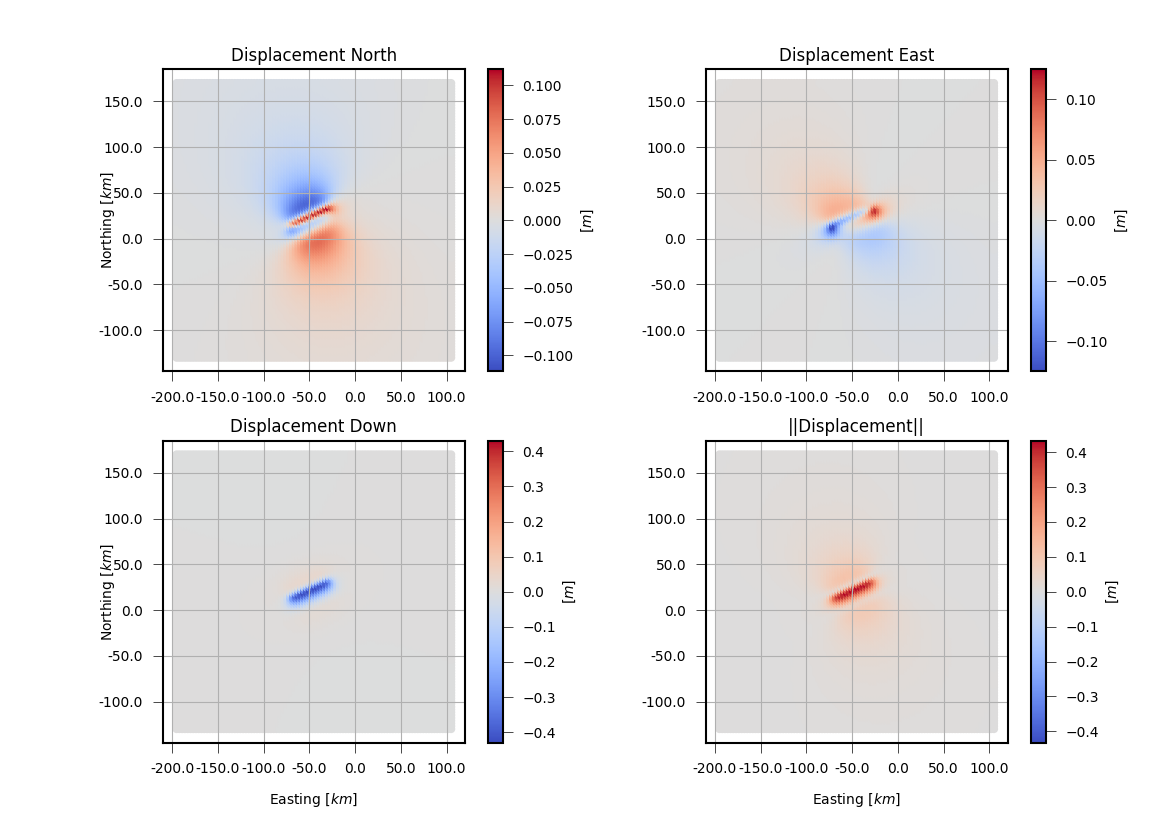
Surface displacements (3 components and absolute value) calculated using a
set of OkadaSource.
Footnotes
Calculate spatial surface displacement using the Pseudo Dynamic Rupture
In this example we create a PseudoDynamicRupture and compute the spatial static displacement at the surface invoked by that rupture [2].
Download gf_forward_pseudo_rupture_static.py
import numpy as num
import os.path as op

from matplotlib import pyplot as plt, cm, colors

from pyrocko import gf

km = 1e3
d2r = num.pi / 180.
r2d = 180. / num.pi

# The store we are going extract data from:
store_id = 'gf_abruzzo_nearfield_vmod_Ameri'

# First, download a Greens Functions store. If you already have one that you
# would like to use, you can skip this step and point the *store_superdirs* in
# the next step to that directory.
if not op.exists(store_id):
    gf.ws.download_gf_store(site='pyrocko', store_id=store_id)

# We need a pyrocko.gf.Engine object which provides us with the traces
# extracted from the store. In this case we are going to use a local
# engine since we are going to query a local store.
engine = gf.LocalEngine(store_superdirs=['.'])

# The dynamic parameter used for discretization of the PseudoDynamicRupture are
# extracted from the stores config file.
store = engine.get_store(store_id)

# Let's define the source now with its extension, orientation etc.
source_params = dict(
    north_shift=2. * km,
    east_shift=2. * km,
    depth=1.0 * km,
    length=6. * km,
    width=6. * km,
    strike=0.,
    dip=80.,
    rake=45.,
    anchor='top',
    decimation_factor=1)

dyn_rupture = gf.PseudoDynamicRupture(
    nx=5,
    ny=5,
    pure_shear=True,
    **source_params)

# Recalculate slip, that rupture magnitude fits given magnitude
magnitude = 6.0
dyn_rupture.rescale_slip(magnitude=magnitude, store=store)

# Get rake out of slip (can differ from traction rake!)
slip = dyn_rupture.get_slip()
source_params['rake'] = num.arctan2(slip[0, 1], slip[0, 0]) * r2d

# Create similar rectangular source model with rake derivded from slip
rect_rupture = gf.RectangularSource(
    magnitude=magnitude,
    **source_params)

# Define static target grid to extract the surface displacement
ngrid = 40

obs_size = 10. * km
ntargets = ngrid**2

norths = num.linspace(-obs_size, obs_size, ngrid) + \
    source_params['north_shift']
easts = num.linspace(-obs_size, obs_size, ngrid) + \
    source_params['east_shift']

norths2d = num.repeat(norths, len(easts))
easts2d = num.tile(easts, len(norths))

static_target = gf.StaticTarget(
    lats=num.ones(norths2d.size) * dyn_rupture.effective_lat,
    lons=num.ones(norths2d.size) * dyn_rupture.effective_lon,
    north_shifts=norths2d,
    east_shifts=easts2d,
    interpolation='nearest_neighbor',
    store_id=store_id)

# Get static surface displacements for rectangular and pseudo dynamic source
result = engine.process(rect_rupture, static_target)

targets_static = result.request.targets_static
synth_disp_rect = result.results_list[0][0].result

result = engine.process(dyn_rupture, static_target)

targets_static = result.request.targets_static
synth_disp_dyn = result.results_list[0][0].result

# Extract static vertical displacement and plot
down_rect = synth_disp_rect['displacement.d']
down_dyn = synth_disp_dyn['displacement.d']
down_diff = down_rect - down_dyn

vabsmax = num.max(num.abs([down_rect, down_dyn, down_diff]))
vmin = -vabsmax
vmax = vabsmax

fig = plt.figure(figsize=(10, 10))
axes = []
for i in [1, 2, 3]:
    axes.append(fig.add_subplot(2, 2, i, aspect=1.0))

cax = fig.add_axes((0.6, 0.125, 0.02, 0.3))

cmap = 'RdBu_r'
norm = colors.Normalize(vmin=vmin, vmax=vmax)

for ax, (down, label) in zip(
        axes[:3],
        zip((down_rect, down_dyn, down_diff),
            (r'$u_{Z, rect}$', r'$u_{Z, dyn}$', r'$\Delta u_{Z}$'))):

    ax.pcolormesh(
        easts/km, norths/km, down.reshape(ngrid, ngrid),
        cmap=cmap, norm=norm, shading='gouraud')

    ax.set_title(label)

axes[1].set_xlabel('Easting [km]')
axes[2].set_xlabel('Easting [km]')
axes[0].set_ylabel('Northing [km]')
axes[2].set_ylabel('Northing [km]')

axes[0].get_xaxis().set_tick_params(
    bottom=True, labelbottom=False, top=False, labeltop=False)

axes[1].get_yaxis().set_tick_params(
    left=True, right=False, labelleft=False, labelright=False)

sm = cm.ScalarMappable(norm=norm, cmap=cmap)
sm.set_array([])  # If not set, an error might be issued

cbar = fig.colorbar(sm, cax=cax)
cbar.ax.set_ylabel('$u$ [m]')

fig.savefig('gf_forward_pseudo_rupture_static.png')

plt.show()
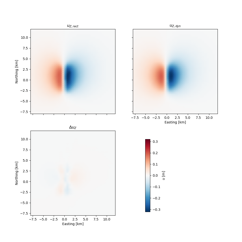
Vertical surface displacements derived from a
PseudoDynamicRupture. They are compared
to vertical static displacements calculated using the
RectangularSource.
Footnotes
Calculate spatial surface displacement and export Kite scenes
We derive InSAR surface deformation targets from Kite scenes. This way we can easily inspect the data and use Kite’s quadtree data sub-sampling and data error variance-covariance estimation calculation.
Download gf_forward_example2_kite.py
import os.path
from kite.scene import Scene, FrameConfig
from pyrocko import gf
import numpy as num

km = 1e3
d2r = num.pi/180.

# Download a Greens Functions store
store_id = 'gf_abruzzo_nearfield_vmod_Ameri'
if not os.path.exists(store_id):
    gf.ws.download_gf_store(site='pyrocko', store_id=store_id)

# Setup the modelling LocalEngine
# *store_superdirs* is a list of directories where to look for GF Stores.
engine = gf.LocalEngine(store_superdirs=['.'])

rect_source = gf.RectangularSource(
    # Geographical position [deg]
    lat=0., lon=0.,
    # Relative cartesian offsets [m]
    north_shift=10*km, east_shift=10*km,
    depth=6.5*km,
    # Dimensions of the fault [m]
    width=5*km, length=8*km,
    strike=104., dip=90., rake=0.,
    # Slip in [m]
    slip=1., anchor='top')

# Define the scene's frame
frame = FrameConfig(
    # Lower left geographical reference [deg]
    llLat=0., llLon=0.,
    # Pixel spacing [m] or [degrees]
    spacing='meter', dE=250, dN=250)

# Resolution of the scene
npx_east = 800
npx_north = 800

# 2D arrays for displacement and look vector
displacement = num.empty((npx_east, npx_north))

# Look vectors
# Theta is elevation angle from horizon
theta = num.full_like(displacement, 48.*d2r)
# Phi is azimuth towards the satellite, counter-clockwise from East
phi = num.full_like(displacement, 23.*d2r)

scene = Scene(
    displacement=displacement,
    phi=phi, theta=theta,
    frame=frame)

# Or just load an existing scene!
# scene = Scene.load('my_scene_asc.npy')

satellite_target = gf.KiteSceneTarget(
    scene,
    store_id=store_id)

# Forward model!
result = engine.process(
    rect_source, satellite_target,
    # Use all available cores
    nthreads=0)

kite_scenes = result.kite_scenes()

# Show the synthetic data in spool
# kite_scenes[0].spool()
Calculate forward model of thrust faulting and display wrapped phase
In this example we compare the synthetic unwappred and wrapped LOS displacements caused by a thrust rupture.
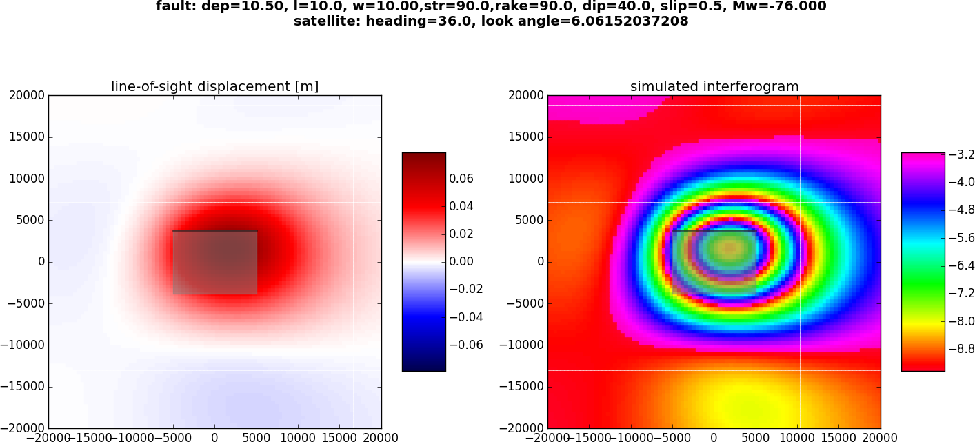
Synthetic LOS displacements from a south-dipping thrust fault. LOS as for Sentinel-1 satellite (Look Angle: 36., Heading:-76). Positive motion toward the satellite. Left: unwrapped phase. Right: Wrapped phase.
Download gf_forward_example3.py
import os.path
import numpy as num
import matplotlib.pyplot as plt
from pyrocko import gf

km = 1e3

# Download a Greens Functions store, programmatically.
store_id = 'gf_abruzzo_nearfield_vmod_Ameri'
if not os.path.exists(store_id):
    gf.ws.download_gf_store(site='pyrocko', store_id=store_id)

# Ignite the LocalEngine and point it to your fomosto store at '.'
engine = gf.LocalEngine(store_superdirs=['.'])

# RectangularSource parameters
strike = 90.
dip = 40.
dep = 10.5*km
leng = 10.*km
wid = 10.*km
rake = 90.
slip = .5

# Magnitude of the event
potency = leng * wid * slip
rigidity = 31.5e9
m0 = potency*rigidity
mw = (2./3) * num.log10(m0) - 6.07

# Define an extended RectangularSource
thrust = gf.RectangularSource(
    north_shift=0., east_shift=0.,
    depth=dep, width=wid, length=leng,
    dip=dip, rake=rake, strike=strike,
    slip=slip)

# Define a grid of targets
# number in east and north directions, and total
ngrid = 40
# ngrid = 90  # for better resolution

# extension from origin in all directions
obs_size = 20.*km
ntargets = ngrid**2

norths = num.linspace(-obs_size, obs_size, ngrid)
easts = num.linspace(-obs_size, obs_size, ngrid)

# make regular grid
norths2d = num.repeat(norths, len(easts))
easts2d = num.tile(easts, len(norths))

# Initialize the SatelliteTarget and set the line of site vectors
# Case example of the Sentinel-1 satellite:
#
# Heading: -166 (anti-clockwise rotation from east)
# Average Look Angle: 36 (from vertical)
heading = -76.
look = 36.
phi = num.empty(ntargets)  # Horizontal LOS from E in anti-clockwise rotation
theta = num.empty(ntargets)  # Vertical LOS from horizontal
phi.fill(num.deg2rad(-90-heading))
theta.fill(num.deg2rad(90.-look))

satellite_target = gf.SatelliteTarget(
    north_shifts=norths2d,
    east_shifts=easts2d,
    tsnapshot=24.*3600.,    # one day
    interpolation='nearest_neighbor',
    phi=phi,
    theta=theta,
    store_id=store_id)

# Forward-modell is performed by calling 'process' on the engine
result = engine.process(thrust, [satellite_target])

# Retrieve synthetic displacements and coordinates from engine's result
# of the first target (it=0)
it = 0
N = result.request.targets[it].coords5[:, 2]
E = result.request.targets[it].coords5[:, 3]
synth_disp = result.results_list[0][it].result

# Fault projection to the surface for plotting
n, e = thrust.outline(cs='xy').T

fig, _ = plt.subplots(1, 2, figsize=(8, 4))
fig.suptitle(
    'fault: dep={:0.2f}, l={}, w={:0.2f},str={},'
    'rake={}, dip={}, slip={}, Mw={:0.3f}\n'
    'satellite: heading={}, look angle={}'
    .format(dep/km, leng/km, wid/km,
            strike, rake, dip, slip, heading, look, mw),
    fontsize=14,
    fontweight='bold')

# Shift the relative LOS displacements
los = synth_disp['displacement.los']
losmax = num.abs(los).max()

# Plot unwrapped LOS displacements
ax = fig.axes[0]
cmap = ax.scatter(
    E, N, c=los,
    s=10., marker='s',
    edgecolor='face',
    cmap=plt.get_cmap('seismic'),
    vmin=-1.*losmax, vmax=1.*losmax)

ax.set_title('line-of-sight displacement [m]')
ax.set_aspect('equal')
ax.set_xlim(-obs_size, obs_size)
ax.set_ylim(-obs_size, obs_size)
# Fault outline
ax.fill(e, n, color=(0.5, 0.5, 0.5), alpha=0.5)
# Underline the tip of the thrust
ax.plot(e[:2], n[:2], linewidth=2., color='black', alpha=0.5)

fig.colorbar(cmap, ax=ax, orientation='vertical', aspect=5, shrink=0.5)

# Simulate a C-band interferogram for this source
c_lambda = 0.056
insar_phase = -num.mod(los, c_lambda/2.)/(c_lambda/2.)*2.*num.pi - num.pi

# Plot wrapped phase
ax = fig.axes[1]
cmap = ax.scatter(
    E, N, c=insar_phase,
    s=10., marker='s',
    edgecolor='face',
    cmap=plt.get_cmap('gist_rainbow'))

ax.set_xlim(-obs_size, obs_size)
ax.set_ylim(-obs_size, obs_size)
ax.set_title('simulated interferogram')
ax.set_aspect('equal')

# plot fault outline
ax.fill(e, n, color=(0.5, 0.5, 0.5), alpha=0.5)
# We outline the top edge of the fault with a thick line
ax.plot(e[:2], n[:2], linewidth=2., color='black', alpha=0.5)

fig.colorbar(cmap, orientation='vertical', shrink=0.5, aspect=5)
plt.show()
Combining dislocation sources
In this example we combine two rectangular sources and plot the forward model in profile.
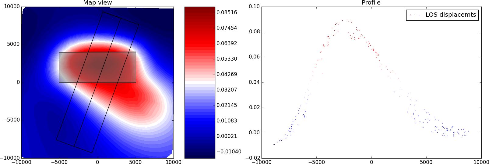
Synthetic LOS displacements from a flower-structure made of one strike-slip fault and one thrust fault. LOS as for Sentinel-1 satellite (Look Angle: 36°, Heading: -76°). Positive motion toward the satellite.
Download gf_forward_example4.py
import os.path
import numpy as num
from pyrocko import gf
from pyrocko.guts import List


class CombiSource(gf.Source):
    '''Composite source model.'''

    discretized_source_class = gf.DiscretizedMTSource

    subsources = List.T(gf.Source.T())

    def __init__(self, subsources=[], **kwargs):

        if subsources:

            lats = num.array(
                [subsource.lat for subsource in subsources], dtype=float)
            lons = num.array(
                [subsource.lon for subsource in subsources], dtype=float)

            assert num.all(lats == lats[0]) and num.all(lons == lons[0])
            lat, lon = lats[0], lons[0]

            # if not same use:
            # lat, lon = center_latlon(subsources)

            depth = float(num.mean([p.depth for p in subsources]))
            t = float(num.mean([p.time for p in subsources]))
            kwargs.update(time=t, lat=float(lat), lon=float(lon), depth=depth)

        gf.Source.__init__(self, subsources=subsources, **kwargs)

    def get_factor(self):
        return 1.0

    def discretize_basesource(self, store, target=None):
        dsources = []
        t0 = self.subsources[0].time
        for sf in self.subsources:
            assert t0 == sf.time
            ds = sf.discretize_basesource(store, target)
            ds.m6s *= sf.get_factor()
            dsources.append(ds)

        return gf.DiscretizedMTSource.combine(dsources)


# Download a Greens Functions store, programmatically.
store_id = 'gf_abruzzo_nearfield_vmod_Ameri'
if not os.path.exists(store_id):
    gf.ws.download_gf_store(site='pyrocko', store_id=store_id)

km = 1e3   # distance in kilometer

# We define a grid for the targets.
left, right, bottom, top = -10*km, 10*km, -10*km, 10*km
ntargets = 1000

# Ignite the LocalEngine and point it to fomosto stores stored on a
# USB stick, for this example we use a static store with id 'static_store'
engine = gf.LocalEngine(store_superdirs=['.'])
store_id = 'gf_abruzzo_nearfield_vmod_Ameri'

# We define two finite sources
# The first one is a purely vertical strike-slip fault
strikeslip = gf.RectangularSource(
    north_shift=0., east_shift=0.,
    depth=6*km, width=4*km, length=10*km,
    dip=90., rake=0., strike=90.,
    slip=1.)

# The second one is a ramp connecting to the root of the strike-slip fault
# ramp north shift (n) and width (w) depend on its dip angle and on
# the strike slip fault width
n, w = 2/num.tan(num.deg2rad(45.)), 2.*(2./(num.sin(num.deg2rad(45.))))
thrust = gf.RectangularSource(
    north_shift=n*km, east_shift=0.,
    depth=6*km, width=w*km, length=10*km,
    dip=45., rake=90., strike=90.,
    slip=0.5)

# We initialize the satellite target and set the line of site vectors
# Case example of the Sentinel-1 satellite:
# Heading: -166 (anti clockwise rotation from east)
# Average Look Angle: 36 (from vertical)
heading = -76
look = 36.
phi = num.empty(ntargets)    # Horizontal LOS from E in anti-clockwise rotation
theta = num.empty(ntargets)  # Vertical LOS from horizontal
phi.fill(num.deg2rad(-90. - heading))
theta.fill(num.deg2rad(90. - look))

satellite_target = gf.SatelliteTarget(
    north_shifts=num.random.uniform(bottom, top, ntargets),
    east_shifts=num.random.uniform(left, right, ntargets),
    tsnapshot=24.*3600.,
    interpolation='nearest_neighbor',
    phi=phi,
    theta=theta,
    store_id=store_id)

# We combine the two sources here
patches = [strikeslip, thrust]
sources = CombiSource(subsources=patches)

# The computation is performed by calling process on the engine
result = engine.process(sources, [satellite_target])


def plot_static_los_profile(result, strike, l, w, x0, y0):  # noqa
    import matplotlib.pyplot as plt
    import matplotlib.cm as cm
    import matplotlib.colors as mcolors
    fig, _ = plt.subplots(1, 2, figsize=(8, 4))

    # strike,l,w,x0,y0: strike, length, width, x, and y position
    # of the profile
    strike = num.deg2rad(strike)
    # We define the parallel and perpendicular vectors to the profile
    s = [num.sin(strike), num.cos(strike)]
    n = [num.cos(strike), -num.sin(strike)]

    # We define the boundaries of the profile
    ypmax, ypmin = l/2, -l/2
    xpmax, xpmin = w/2, -w/2

    # We define the corners of the profile
    xpro, ypro = num.zeros((7)), num.zeros((7))
    xpro[:] = x0-w/2*s[0]-l/2*n[0], x0+w/2*s[0]-l/2*n[0], \
        x0+w/2*s[0]+l/2*n[0], x0-w/2*s[0]+l/2*n[0], x0-w/2*s[0]-l/2*n[0], \
        x0-l/2*n[0], x0+l/2*n[0]

    ypro[:] = y0-w/2*s[1]-l/2*n[1], y0+w/2*s[1]-l/2*n[1], \
        y0+w/2*s[1]+l/2*n[1], y0-w/2*s[1]+l/2*n[1], y0-w/2*s[1]-l/2*n[1], \
        y0-l/2*n[1], y0+l/2*n[1]

    # We get the forward model from the engine
    N = result.request.targets[0].coords5[:, 2]
    E = result.request.targets[0].coords5[:, 3]
    result = result.results_list[0][0].result

    # We first plot the surface displacements in map view
    ax = fig.axes[0]
    los = result['displacement.los']
    levels = num.linspace(los.min(), los.max(), 50)

    cmap = ax.tricontourf(E, N, los, cmap=plt.get_cmap('seismic'),
                          levels=levels)

    for sourcess in patches:
        fn, fe = sourcess.outline(cs='xy').T
        ax.fill(fe, fn, color=(0.5, 0.5, 0.5), alpha=0.5)
        ax.plot(fe[:2], fn[:2], linewidth=2., color='black', alpha=0.5)

    # We plot the limits of the profile in map view
    ax.plot(xpro[:], ypro[:], color='black', lw=1.)
    # plot colorbar
    fig.colorbar(cmap, ax=ax, orientation='vertical', aspect=5)
    ax.set_title('Map view')
    ax.set_aspect('equal')

    # We plot displacements in profile
    ax = fig.axes[1]
    # We compute the perpendicular and parallel components in the profile basis
    yp = (E-x0)*n[0]+(N-y0)*n[1]
    xp = (E-x0)*s[0]+(N-y0)*s[1]
    los = result['displacement.los']

    # We select data encompassing the profile
    index = num.nonzero(
        (xp > xpmax) | (xp < xpmin) | (yp > ypmax) | (yp < ypmin))

    ypp, losp = num.delete(yp, index), \
        num.delete(los, index)

    # We associate the same color scale to the scatter plot
    norm = mcolors.Normalize(vmin=los.min(), vmax=los.max())
    m = cm.ScalarMappable(norm=norm, cmap=plt.get_cmap('seismic'))
    facelos = m.to_rgba(losp)
    ax.scatter(
        ypp, losp,
        s=0.3, marker='o', color=facelos, label='LOS displacements')

    ax.legend(loc='best')
    ax.set_title('Profile')

    plt.show()


plot_static_los_profile(result, 110., 18*km, 5*km, 0., 0.)
Modelling viscoelastic static displacement
In this advanced example we leverage the viscoelastic forward modelling capabilities of the psgrn_pscmp backend.
Viscoelastic static GF store forward-modeling the transient effects of a deep dislocation source, mimicking a transform plate boundary. Together with a shallow seismic source. The cross denotes the tracked pixel location. (Top) Displacement of the tracked pixel in time.
The static store has to be setup with Burger material describing the viscoelastic properties of the medium, see this config for the fomosto store:
Note
Static stores define the sampling rate in Hz.
sampling_rate: 1.157e-06 Hz is a sampling rate of 10 days!
--- !pf.ConfigTypeA
id: static_t
modelling_code_id: psgrn_pscmp.2008a
regions: []
references: []
earthmodel_1d: |2
      0.             2.5            1.2            2.1           50.            50.
      1.             2.5            1.2            2.1           50.            50.
      1.             6.2            3.6            2.8          600.           400.
     17.             6.2            3.6            2.8          600.           400.
     17.             6.6            3.7            2.9         1432.           600.
     32.             6.6            3.7            2.9         1432.           600.
     32.             7.3            4.             3.1         1499.           600.            1e30            1e20           1.
     41.             7.3            4.             3.1         1499.           600.            1e30            1e20           1.
  mantle
     41.             8.2            4.7            3.4         1370.           600.            1e19            5e17           1.
     91.             8.2            4.7            3.4         1370.           600.            1e19            5e17           1.
sample_rate: 1.1574074074074074e-06
component_scheme: elastic10
tabulated_phases: []
ncomponents: 10
receiver_depth: 0.0
source_depth_min: 0.0
source_depth_max: 40000.0
source_depth_delta: 500.0
distance_min: 0.0
distance_max: 150000.0
distance_delta: 1000.0
In the extra/psgrn_pscmp configruation file we have to define the timespan from tmin_days to tmax_days, covered by the sampling_rate (see above)
--- !pf.PsGrnPsCmpConfig
tmin_days: 0.0
tmax_days: 600.0
gf_outdir: psgrn_functions
psgrn_config: !pf.PsGrnConfig
  version: 2008a
  sampling_interval: 1.0
  gf_depth_spacing: -1.0
  gf_distance_spacing: -1.0
  observation_depth: 0.0
pscmp_config: !pf.PsCmpConfig
  version: 2008a
  observation: !pf.PsCmpScatter {}
  rectangular_fault_size_factor: 1.0
  rectangular_source_patches: []
Download gf_forward_viscoelastic.py
'''
An advanced example requiring a viscoelastic static store.
See https://pyrocko.org for detailed instructions.
'''
import logging
import os.path as op
import matplotlib.pyplot as plt
from matplotlib.animation import FuncAnimation
from matplotlib.ticker import FuncFormatter

import numpy as num
from pyrocko import gf

logging.basicConfig(level=logging.INFO)
logger = logging.getLogger('static-viscoelastic')

km = 1e3
d2r = num.pi/180.
store_id = 'static_t'

day = 3600*24

engine = gf.LocalEngine(store_superdirs=['.'])

ngrid = 100

extent = (-75*km, 75*km)
dpx = abs((extent[0] - extent[1]) / ngrid)

easts = num.linspace(*extent, ngrid)
norths = num.linspace(*extent, ngrid)
east_shifts = num.tile(easts, ngrid)
north_shifts = num.repeat(norths, ngrid)

look = 23.
heading = -76.  # descending
npx = int(ngrid**2)

tmax = 1000*day
t_eq = 200*day
nsteps = 200

dt = tmax / nsteps

satellite_target = gf.SatelliteTarget(
    east_shifts=east_shifts,
    north_shifts=north_shifts,
    phi=num.full(npx, d2r*(90.-look)),
    theta=num.full(npx, d2r*(-90.-heading)),
    interpolation='nearest_neighbor')

creep_source = gf.RectangularSource(
    lat=0., lon=0.,
    north_shift=3*km, east_shift=0.,
    depth=25*km,
    width=15*km, length=80*km,
    strike=100., dip=90., rake=0.,
    slip=0.08, anchor='top',
    decimation_factor=4)

coseismic_sources = gf.RectangularSource(
    lat=0., lon=0.,
    north_shift=3*km, east_shift=0.,
    depth=15*km,
    width=10*km, length=60*km,
    strike=100., dip=90., rake=0.,
    slip=.5, anchor='top',
    decimation_factor=4,
    time=t_eq)

targets = []
for istep in range(nsteps):
    satellite_target = gf.SatelliteTarget(
        east_shifts=east_shifts,
        north_shifts=north_shifts,
        phi=num.full(npx, d2r*(90.-look)),
        theta=num.full(npx, d2r*(-90.-heading)),
        interpolation='nearest_neighbor',
        tsnapshot=dt*istep)
    targets.append(satellite_target)


def get_displacement(sources, targets, component='los'):
    result = engine.process(
        sources, targets,
        nthreads=0)

    static_results = result.static_results()
    nres = len(static_results)

    res_arr = num.empty((nres, ngrid, ngrid))

    for ires, res in enumerate(static_results):
        res_arr[ires] = res.result['displacement.%s' % component]\
            .reshape(ngrid, ngrid)
    return res_arr


component = 'los'
fn = 'displacement_%s' % component

# Use cached displacements
if not op.exists('%s.npy' % fn):
    logger.info('Calculating scenario for %s.npy ...', fn)
    displacement_creep = get_displacement(
        creep_source, satellite_target, component)[0]
    displacement_creep /= 365.

    displacement = get_displacement(coseismic_sources, targets, component)

    for istep in range(nsteps):
        displacement[istep] += displacement_creep * (dt / day) * istep

    num.save(fn, displacement)
else:
    logger.info('Loading scenario data from %s.npy ...', fn)
    displacement = num.load('%s.npy' % fn)

if False:
    fig = plt.figure()
    ax = fig.gca()

    for ipx in range(ngrid)[::10]:
        for ipy in range(ngrid)[::10]:
            ax.plot(displacement[:, ipx, ipy], alpha=.3, color='k')

    plt.show()


sample_point = (-20.*km, -27.*km)
sample_idx = (int(sample_point[0] / dpx), int(sample_point[1] / dpx))

fig, (ax_time, ax_u) = plt.subplots(
    2, 1, gridspec_kw={'height_ratios': [1, 4]})
fig.set_size_inches(10, 8)
ax_u = fig.gca()

vrange = num.abs(displacement).max()
colormesh = ax_u.pcolormesh(
    easts, norths, displacement[80],
    cmap='seismic', vmin=-vrange, vmax=vrange, shading='gouraud',
    animated=True)

smpl_point = ax_u.scatter(
    *sample_point, marker='x', color='black', s=30, zorder=30)

time_label = ax_u.text(.95, .05, '0 days', ha='right', va='bottom',
                       alpha=.5, transform=ax_u.transAxes, zorder=20)

# cbar = fig.colorbar(img)
# cbar.set_label('Displacment %s [m]', )

ax_u.set_xlabel('Easting [km]')
ax_u.set_ylabel('Northing [km]')

km_formatter = FuncFormatter(lambda x, pos: x / km)
ax_u.xaxis.set_major_formatter(km_formatter)
ax_u.yaxis.set_major_formatter(km_formatter)

ax_time.set_title('%s Displacement' % component.upper())
urange = (displacement[:, sample_idx[0], sample_idx[1]].min() * 1.05,
          displacement[:, sample_idx[0], sample_idx[1]].max() * 1.05)
ut = ax_time.plot([], [], color='black')[0]
ax_time.axvline(x=t_eq + dt, linestyle='--', color='red', alpha=.5)

day_formatter = FuncFormatter(lambda x, pos: int(x / day))
ax_time.xaxis.set_major_formatter(day_formatter)
ax_time.set_xlim(0., tmax)
ax_time.set_ylim(*urange)

ax_time.set_xlabel('Days')
ax_time.set_ylabel('Displacement [m]')
ax_time.grid(alpha=.3)


def animation_update(frame):
    colormesh.set_array(displacement[frame].ravel())
    time_label.set_text('%d days' % int(frame * (dt / day)))

    ut.set_xdata(num.arange(frame) * dt)
    ut.set_ydata(displacement[:frame, sample_idx[0], sample_idx[1]])

    return colormesh, smpl_point, time_label, ut


ani = FuncAnimation(
    fig, animation_update, frames=nsteps, interval=30, blit=True)
# plt.show()

logger.info('Saving animation...')
ani.save('viscoelastic-response.mp4', writer='ffmpeg')
Creating a custom Source Time Function (STF)
Basic example how to create a custom STF class, creating a linearly decreasing ramp excitation.
Download gf_custom_stf.py
from pyrocko.gf import STF
from pyrocko.guts import Float
import numpy as num


class LinearRampSTF(STF):
    '''Linearly decreasing ramp from maximum amplitude to zero.'''

    duration = Float.T(
        default=0.0,
        help='baseline of the ramp')

    anchor = Float.T(
        default=0.0,
        help='anchor point with respect to source-time: ('
             '-1.0: left -> source duration [0, T] ~ hypocenter time, '
             ' 0.0: center -> source duration [-T/2, T/2] ~ centroid time, '
             '+1.0: right -> source duration [-T, 0] ~ rupture end time)')

    def discretize_t(self, deltat, tref):
        # method returns discrete times and the respective amplitudes
        tmin_stf = tref - self.duration * (self.anchor + 1.) * 0.5
        tmax_stf = tref + self.duration * (1. - self.anchor) * 0.5
        tmin = round(tmin_stf / deltat) * deltat
        tmax = round(tmax_stf / deltat) * deltat
        nt = int(round((tmax - tmin) / deltat)) + 1
        times = num.linspace(tmin, tmax, nt)
        if nt > 1:
            amplitudes = num.linspace(1., 0., nt)
            amplitudes /= num.sum(amplitudes)  # normalise to keep moment
        else:
            amplitudes = num.ones(1)

        return times, amplitudes

    def base_key(self):
        # method returns STF name and the values
        return (self.__class__.__name__, self.duration, self.anchor)