
Traveltime calculation and raytracing
Calculate traveltimes in layered media
Here we will excercise two example how to calculate traveltimes for the phases P and Pg for different earth velocity models.
- Modules covered in this example:
-
The first example is minimalistic and will give you a simple traveltime table.
Download cake_ray_tracing.py
'''
Calculate P-phase arrivals.
'''

from pyrocko import cake
import numpy as num

km = 1000.

# Load builtin 'prem-no-ocean' model (medium resolution)
model = cake.load_model('prem-no-ocean.m')

# Source depth [m].
source_depth = 300. * km

# Distances as a numpy array [deg].
distances = num.linspace(1500, 3000, 16)*km * cake.m2d

# Define the phase to use.
Phase = cake.PhaseDef('P')

# calculate distances and arrivals and print them:
print('distance [km]      time [s]')
for arrival in model.arrivals(distances, phases=Phase, zstart=source_depth):
    print('%13g %13g' % (arrival.x*cake.d2m/km, arrival.t))
The second code snippet includes some lines to plot a simple traveltime figure.
Download cake_ray_tracing.py
import numpy as num
from matplotlib import pyplot as plt

from pyrocko.plot import mpl_init, mpl_margins, mpl_papersize
from pyrocko import cake

fontsize = 9.
km = 1000.

mod = cake.load_model('ak135-f-continental.m')

phases = cake.PhaseDef.classic('Pg')
source_depth = 20.*km

distances = num.linspace(100.*km, 1000.*km, 100)

data = []
for distance in distances:
    rays = mod.arrivals(
        phases=phases, distances=[distance*cake.m2d], zstart=source_depth)
    for ray in rays[:1]:
        data.append((distance, ray.t))

phase_distances, phase_time = num.array(data, dtype=float).T

# Plot the arrival times
mpl_init(fontsize=fontsize)
fig = plt.figure(figsize=mpl_papersize('a5', 'landscape'))
labelpos = mpl_margins(fig, w=7., h=5., units=fontsize)
axes = fig.add_subplot(1, 1, 1)
labelpos(axes, 2., 1.5)

axes.set_xlabel('Distance [km]')
axes.set_ylabel('Time [s]')

axes.plot(phase_distances/km, phase_time, 'o', ms=3., color='black')

fig.savefig('cake_first_arrivals.pdf')
Calculate traveltimes in heterogeneous media
These examples demonstrate how to use the pyrocko.modelling.eikonal
module to calculate first arrivals in heterogenous media.
import numpy as num
from matplotlib import pyplot as plt
from pyrocko.modelling import eikonal

km = 1000.
nx, ny = 1500, 500                # grid size
delta = 90*km / float(nx)         # grid spacing
source_x, source_y = 0.0, 15*km   # source position

# Indexing arrays
x = num.arange(nx) * delta - 2*km
y = num.arange(ny) * delta
x2 = x[num.newaxis, :]
y2 = y[:, num.newaxis]

# Define layers with different speeds, roughly representing a crustal model.
speeds = num.ones((ny, nx))
nlayer = ny // 5
speeds[0*nlayer:1*nlayer, :] = 2500.
speeds[1*nlayer:2*nlayer, :] = 3500.
speeds[2*nlayer:3*nlayer, :] = 5000.
speeds[3*nlayer:4*nlayer, :] = 6000.
speeds[4*nlayer:, :] = 8000.

# Seeding points have non-negative times. Here we simply set one grid node to
# zero. The solution to the eikonal equation is computed at all nodes where
# times < 0.
times = num.zeros((ny, nx)) - 1.0
times[int(round(source_y/delta)), int(round((source_x-x[0])//delta))] = 0.0

# Solve eikonal equation.
eikonal.eikonal_solver_fmm_cartesian(speeds, times, delta)

# Plot
fig = plt.figure(figsize=(9.0, 4.0))

axes = fig.add_subplot(1, 1, 1, aspect=1.0)
axes.contourf(x/km, y/km, times)
axes.invert_yaxis()
axes.contourf(x/km, y/km, speeds, alpha=0.1, cmap='gray')
axes.plot(source_x/km, source_y/km, '*', ms=20, color='white')
axes.set_xlabel('Distance [km]')
axes.set_ylabel('Depth [km]')
# fig.savefig('eikonal_example1.png')
plt.show()
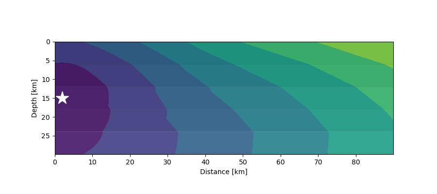
First arrivals (contours) from a seismic source (star) at 15 km depth in a 5-layer crustal model where velocities increase with depth.
import numpy as num
from matplotlib import pyplot as plt
from pyrocko.modelling import eikonal

km = 1000.
nx, ny = 1000, 500          # grid size
delta = 20*km / float(nx)   # drid spacing

# Indexing arrays
x = num.arange(nx) * delta - 10.0
y = num.arange(ny) * delta
x2 = x[num.newaxis, :]
y2 = y[:, num.newaxis]

# Define layers and circles with different speeds, roughly representing a case
# with two layers and intrusions.
speeds = num.ones((ny, nx))
r1 = num.sqrt((x2-0*km)**2 + (y2-2*km)**2)
r2 = num.sqrt((x2-12*km)**2 + (y2-0*km)**2)
nlayer = ny // 5
speeds[r1 < 4*km] = 2.0
speeds[r2 < 4*km] = 0.7
speeds[:3*nlayer, :] *= 0.5

# Seeding points have non-negative times. Here we
times = num.zeros((ny, nx)) - 1.0
times[-1, :] = (x-num.min(x)) * 0.1

# Solve eikonal equation.
eikonal.eikonal_solver_fmm_cartesian(speeds, times, delta)

# Plot
fig = plt.figure(figsize=(9.0, 4.0))

axes = fig.add_subplot(1, 1, 1, aspect=1.0)
axes.contourf(x/km, y/km, times)
axes.invert_yaxis()
axes.contourf(x/km, y/km, speeds, alpha=0.1, cmap='gray')
axes.set_xlabel('Distance [km]')
axes.set_ylabel('Depth [km]')
# fig.savefig('eikonal_example2.png')
plt.show()
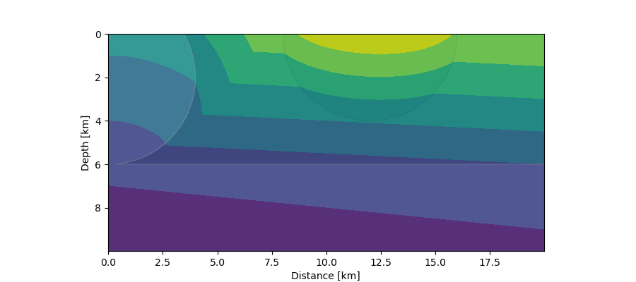
First arrivals (contours) from a distant seismic source in a 2-layer crustal model with intrusions. The planar wave front entering from below is simulated by a source at 10 km depth moving quickly from left to right with a given constant speed.
Traveltime table interpolation
This example demonstrates how to interpolate and query traveltime tables.
- Classes covered in this example:
pyrocko.spit.SPTree(interpolation of traveltime tables)pyrocko.gf.meta.TPDef(phase definitions)pyrocko.gf.meta.Timing(onset definition to query the travel time tables)
Download cake_raytracing.py
import numpy as num
import matplotlib.pyplot as plt
from pyrocko import spit, cake
from pyrocko.gf import meta


# Define a list of phases.
phase_defs = [meta.TPDef(id='stored:depth_p', definition='p'),
              meta.TPDef(id='stored:P', definition='P')]

# Load a velocity model. In this example use the default AK135.
mod = cake.load_model()

# Time and space tolerance thresholds defining the accuracy of the
# :py:class:`pyrocko.spit.SPTree`.
t_tolerance = 0.1                           # in seconds
x_tolerance = num.array((500., 500.))       # in meters

# Boundaries of the grid.
xmin = 0.
xmax = 20000
zmin = 0.
zmax = 11000
x_bounds = num.array(((xmin, xmax), (zmin, zmax)))

# In this example the receiver is located at the surface.
receiver_depth = 0.

interpolated_tts = {}

for phase_def in phase_defs:
    v_horizontal = phase_def.horizontal_velocities

    def evaluate(args):
        '''Calculate arrival using source and receiver location
        defined by *args*. To be evaluated by the SPTree instance.'''
        source_depth, x = args

        t = []

        # Calculate arrivals
        rays = mod.arrivals(
            phases=phase_def.phases,
            distances=[x*cake.m2d],
            zstart=source_depth,
            zstop=receiver_depth)

        for ray in rays:
            t.append(ray.t)

        for v in v_horizontal:
            t.append(x/(v*1000.))
        if t:
            return min(t)
        else:
            return None

    # Creat a :py:class:`pyrocko.spit.SPTree` interpolator.
    sptree = spit.SPTree(
        f=evaluate,
        ftol=t_tolerance,
        xbounds=x_bounds,
        xtols=x_tolerance)

    # Store the result in a dictionary which is later used to retrieve an
    # SPTree (value) for each phase_id (key).
    interpolated_tts[phase_def.id] = sptree

    # Dump the sptree for later reuse:
    sptree.dump(filename='sptree_%s.yaml' % phase_def.id.split(':')[1])

# Define a :py:class:`pyrocko.gf.meta.Timing` instance.
timing = meta.Timing('first(depth_p|P)')


# If only one interpolated onset is need at a time you can retrieve
# that value as follows:
# First argument has to be a function which takes a requested *phase_id*
# and returns the associated :py:class:`pyrocko.spit.SPTree` instance.
# Second argument is a tuple of distance and source depth.
z_want = 5000.
x_want = 2000.
one_onset = timing.evaluate(lambda x: interpolated_tts[x],
                            (z_want, x_want))
print('a single arrival: ', one_onset)


# But if you have many locations for which you would like to calculate the
# onset time the following is the preferred way as it is much faster
# on large coordinate arrays.
# x_want is now an array of 1000 distances
x_want = num.linspace(0, xmax, 1000)

# Coords is set up of distances-depth-pairs
coords = num.array((x_want, num.tile(z_want, x_want.shape))).T

# *interpolate_many* then interpolates onset times for each of these
# pairs.
tts = interpolated_tts['stored:depth_p'].interpolate_many(coords)

# Plot distance vs. onset time
plt.plot(x_want, tts, '.')
plt.xlabel('Distance [m]')
plt.ylabel('Travel Time [s]')
plt.show()