Plotting functions

Generating topographic maps with automap

The pyrocko.plot.automap module provides a painless and clean interface for the Generic Mapping Tool (GMT) [1].

Classes covered in these examples:

• pyrocko.plot.automap.Map

For details on our approach in calling GMT from Python:

• GmtPy - A Python interface to GMT 4/5

Note

To retain PDF transparency in gmtpy use save(psconvert=True).

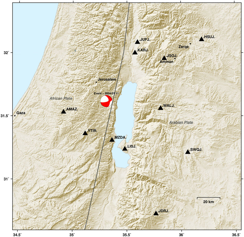
Topographic map of Dead Sea basin

This example demonstrates how to create a map of the Dead Sea area with largest cities, topography and gives a hint on how to access genuine GMT methods.

Download automap_example.py

Station file used in the example: stations_deadsea.pf

from pyrocko.plot.automap import Map
from pyrocko.example import get_example_data
from pyrocko import model
from pyrocko import moment_tensor as pmt
from pyrocko.plot import gmtpy

gmtpy.check_have_gmt()

# Download example data
get_example_data('stations_deadsea.pf')
get_example_data('deadsea_events_1976-2017.txt')

# Generate the basic map
m = Map(
    lat=31.5,
    lon=35.5,
    radius=150000.,
    width=30., height=30.,
    show_grid=False,
    show_topo=True,
    color_dry=(238, 236, 230),
    topo_cpt_wet='light_sea_uniform',
    topo_cpt_dry='light_land_uniform',
    illuminate=True,
    illuminate_factor_ocean=0.15,
    show_rivers=False,
    show_plates=True)

# Draw some larger cities covered by the map area
m.draw_cities()

# Generate with latitute, longitude and labels of the stations
stations = model.load_stations('stations_deadsea.pf')
lats = [s.lat for s in stations]
lons = [s.lon for s in stations]
labels = ['.'.join(s.nsl()) for s in stations]

# Stations as black triangles. Genuine GMT commands can be parsed by the maps'
# gmt attribute. Last argument of the psxy function call pipes the maps'
# pojection system.
m.gmt.psxy(in_columns=(lons, lats), S='t20p', G='black', *m.jxyr)

# Station labels
for i in range(len(stations)):
    m.add_label(lats[i], lons[i], labels[i])


# Load events from catalog file (generated using catalog.GlobalCMT()
# download from www.globalcmt.org)
# If no moment tensor is provided in the catalogue, the event is plotted
# as a red circle. Symbol size relative to magnitude.

events = model.load_events('deadsea_events_1976-2017.txt')
beachball_symbol = 'd'
factor_symbl_size = 5.0
for ev in events:
    mag = ev.magnitude
    if ev.moment_tensor is None:
        ev_symb = 'c'+str(mag*factor_symbl_size)+'p'
        m.gmt.psxy(
            in_rows=[[ev.lon, ev.lat]],
            S=ev_symb,
            G=gmtpy.color('scarletred2'),
            W='1p,black',
            *m.jxyr)
    else:
        devi = ev.moment_tensor.deviatoric()
        beachball_size = mag*factor_symbl_size
        mt = devi.m_up_south_east()
        mt = mt / ev.moment_tensor.scalar_moment() \
            * pmt.magnitude_to_moment(5.0)
        m6 = pmt.to6(mt)
        data = (ev.lon, ev.lat, 10) + tuple(m6) + (1, 0, 0)

        if m.gmt.is_gmt5():
            kwargs = dict(
                M=True,
                S='%s%g' % (beachball_symbol[0], (beachball_size) / gmtpy.cm))
        else:
            kwargs = dict(
                S='%s%g' % (beachball_symbol[0],
                            (beachball_size)*2 / gmtpy.cm))

        m.gmt.psmeca(
            in_rows=[data],
            G=gmtpy.color('chocolate1'),
            E='white',
            W='1p,%s' % gmtpy.color('chocolate3'),
            *m.jxyr,
            **kwargs)

m.save('automap_deadsea.png')

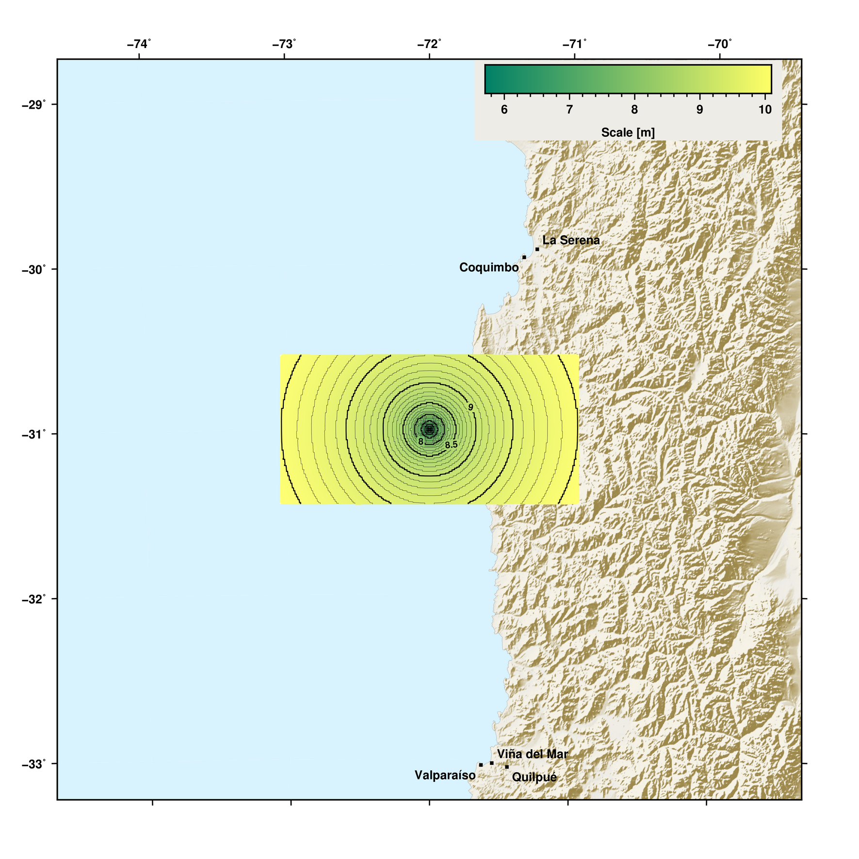
Map with gridded data

This example demonstrates how to create a map using GMT methods and plotting spatial gridded data on it.

Download automap_example2.py

import os

import numpy as num
from scipy.interpolate import RegularGridInterpolator as scrgi

from pyrocko.plot.automap import Map
from pyrocko.plot import gmtpy
import pyrocko.orthodrome as otd

gmtpy.check_have_gmt()
gmt = gmtpy.GMT()

km = 1000.

# Generate the basic map
lat = -31.
lon = -72.
m = Map(
    lat=lat,
    lon=lon,
    radius=250000.,
    width=30., height=30.,
    show_grid=False,
    show_topo=True,
    color_dry=(238, 236, 230),
    topo_cpt_wet='light_sea_uniform',
    topo_cpt_dry='light_land_uniform',
    illuminate=True,
    illuminate_factor_ocean=0.15,
    show_rivers=False,
    show_plates=True)

# Draw some larger cities covered by the map area
m.draw_cities()

# Create grid and data
x = num.linspace(-100., 100., 200) * km
y = num.linspace(-50., 50., 100) * km
yy, xx = num.meshgrid(y, x)

data = num.log10(xx**2 + yy**2)


def extend_1d_coordinate_array(array):
    '''
    Extend 1D coordinate array for gridded data, that grid corners are plotted
    right
    '''
    dx = array[1] - array[0]

    out = num.zeros(array.shape[0] + 2)
    out[1:-1] = array.copy()
    out[0] = array[0] - dx / 2.
    out[-1] = array[-1] + dx / 2.

    return out


def extend_2d_data_array(array):
    '''
    Extend 2D data array for gridded data, that grid corners are plotted
    right
    '''
    out = num.zeros((array.shape[0] + 2, array.shape[1] + 2))
    out[1:-1, 1:-1] = array
    out[1:-1, 0] = array[:, 0]
    out[1:-1, -1] = array[:, -1]
    out[0, 1:-1] = array[0, :]
    out[-1, 1:-1] = array[-1, :]

    for i, j in zip([-1, -1, 0, 0], [-1, 0, -1, 0]):
        out[i, j] = array[i, j]

    return out


def tile_to_length_width(m, ref_lat, ref_lon):
    '''
    Transform grid tile (lat, lon) to easting, northing for data interpolation
    '''
    t, _ = m._get_topo_tile('land')
    grid_lats = t.y()
    grid_lons = t.x()

    meshgrid_lons, meshgrid_lats = num.meshgrid(grid_lons, grid_lats)

    grid_northing, grid_easting = otd.latlon_to_ne_numpy(
        ref_lat, ref_lon, meshgrid_lats.flatten(), meshgrid_lons.flatten())

    return num.hstack((
        grid_easting.reshape(-1, 1), grid_northing.reshape(-1, 1)))


def data_to_grid(m, x, y, data):
    '''
    Create data grid from data and coordinate arrays
    '''
    assert data.shape == (x.shape[0], y.shape[0])

    # Extend grid coordinate and data arrays to plot grid corners right
    x_ext = extend_1d_coordinate_array(x)
    y_ext = extend_1d_coordinate_array(y)
    data_ext = extend_2d_data_array(data)

    # Create grid interpolator based on given coordinates and data
    interpolator = scrgi(
        (x_ext, y_ext),
        data_ext,
        bounds_error=False,
        method='nearest')

    # Interpolate on topography grid from the map
    points_out = tile_to_length_width(m=m, ref_lat=lat, ref_lon=lon)

    t, _ = m._get_topo_tile('land')
    t.data = num.zeros_like(t.data, dtype=float)
    t.data[:] = num.nan

    t.data = interpolator(points_out).reshape(t.data.shape)

    # Save grid as grd-file
    gmtpy.savegrd(t.x(), t.y(), t.data, filename='temp.grd', naming='lonlat')


# Create data grid file
data_to_grid(m, x, y, data)

# Create appropiate colormap
increment = (num.max(data) - num.min(data)) / 20.
gmt.makecpt(
    C='0/127.6/102,255/255/102',
    T='%g/%g/%g' % (num.min(data), num.max(data), increment),
    Z=True,
    out_filename='my_cpt.cpt',
    suppress_defaults=True)

# Plot grid image
m.gmt.grdimage(
    'temp.grd',
    C='my_cpt.cpt',
    E='200',
    I='0.1',
    Q=True,
    n='+t0.15',
    *m.jxyr)

# Plot corresponding contour
m.gmt.grdcontour(
    'temp.grd',
    A='0.5',
    C='0.1',
    S='10',
    W='a1.0p',
    *m.jxyr)

# Plot color scake
m.gmt.psscale(
    B='af+lScale [m]',
    C='my_cpt.cpt',
    D='jTR+o1.05c/0.2c+w10c/1c+h',
    F='+g238/236/230',
    *m.jxyr)

# Save plot
m.save('automap_chile.png', resolution=150)

# Clear temporary files
os.remove('temp.grd')
os.remove('my_cpt.cpt')

Footnotes

[1]

Wessel, P., W. H. F. Smith, R. Scharroo, J. F. Luis, and F. Wobbe, Generic Mapping Tools: Improved version released, EOS Trans. AGU, 94, 409-410, 2013.

Plotting beachballs (focal mechanisms)

Classes covered in these examples:

• pyrocko.plot.beachball (visual representation of a focal mechanism)

• pyrocko.moment_tensor (a 3x3 matrix representation of an earthquake source)

• pyrocko.gf.seismosizer.DCSource (a representation of a double couple source object),

• pyrocko.gf.seismosizer.RectangularExplosionSource (a representation of a rectangular explosion source),

• pyrocko.gf.seismosizer.CLVDSource (a representation of a compensated linear vector dipole source object)

• pyrocko.gf.seismosizer.DoubleDCSource (a representation of a double double-couple source object).

Beachballs from moment tensors

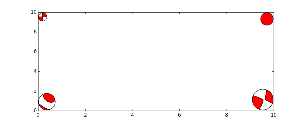
Here we create random moment tensors and plot their beachballs.

Download beachball_example01.py

import random
import logging
from matplotlib import pyplot as plt
from pyrocko import moment_tensor as pmt
from pyrocko import util
from pyrocko.plot import beachball

''' Beachball Copacabana '''

logger = logging.getLogger('pyrocko.examples.beachball_example01')

util.setup_logging()

fig = plt.figure(figsize=(10., 4.))
fig.subplots_adjust(left=0., right=1., bottom=0., top=1.)
axes = fig.add_subplot(1, 1, 1)

for i in range(200):

    # create random moment tensor
    mt = pmt.MomentTensor.random_mt()

    try:
        # create beachball from moment tensor
        beachball.plot_beachball_mpl(
            mt, axes,
            # type of beachball: deviatoric, full or double couple (dc)
            beachball_type='full',
            size=random.random()*120.,
            position=(random.random()*10., random.random()*10.),
            alpha=random.random(),
            linewidth=1.0)

    except beachball.BeachballError as e:
        logger.error('%s for MT:\n%s' % (e, mt))

axes.set_xlim(0., 10.)
axes.set_ylim(0., 10.)
axes.set_axis_off()
fig.savefig('beachball-example01.pdf')

plt.show()

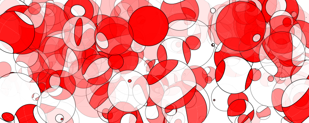
An artistic display of focal mechanisms drawn by classes pyrocko.plot.beachball and pyrocko.moment_tensor.

This example shows how to plot a full, a deviatoric and a double-couple beachball for a moment tensor.

Download beachball_example03.py

from matplotlib import pyplot as plt
from pyrocko import moment_tensor as pmt
from pyrocko import plot
from pyrocko.plot import beachball


fig = plt.figure(figsize=(4., 2.))
fig.subplots_adjust(left=0., right=1., bottom=0., top=1.)
axes = fig.add_subplot(1, 1, 1)
axes.set_xlim(0., 4.)
axes.set_ylim(0., 2.)
axes.set_axis_off()

for i, beachball_type in enumerate(['full', 'deviatoric', 'dc']):
    beachball.plot_beachball_mpl(
            pmt.as_mt((124654616., 370943136., -6965434.0,
                       553316224., -307467264., 84703760.0)),
            axes,
            beachball_type=beachball_type,
            size=60.,
            position=(i+1, 1),
            color_t=plot.mpl_color('scarletred2'),
            linewidth=1.0)

fig.savefig('beachball-example03.pdf')
plt.show()

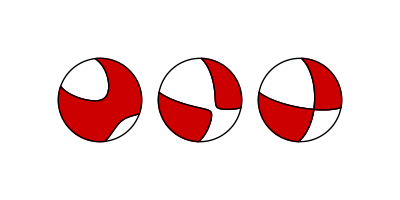
The three types of beachballs that can be plotted through pyrocko.

Beachballs from source objects

This example shows how to add beachballs of various sizes to the corners of a plot by obtaining the moment tensor from four different source object types: pyrocko.gf.seismosizer.DCSource (upper left), pyrocko.gf.seismosizer.RectangularExplosionSource (upper right), pyrocko.gf.seismosizer.CLVDSource (lower left) and pyrocko.gf.seismosizer.DoubleDCSource (lower right).

Creating the beachball this ways allows for finer control over their location based on their size (in display units) which allows for a round beachball even if the axis are not 1:1.

Download beachball_example02.py

from matplotlib import transforms, pyplot as plt
from pyrocko import gf
from pyrocko.plot import beachball


# create source object
source1 = gf.DCSource(depth=35e3, strike=0., dip=90., rake=0.)

# set size of beachball
sz = 20.
# set beachball offset in points (one point from each axis)
szpt = (sz / 2.) / 72. + 1. / 72.

fig = plt.figure(figsize=(10., 4.))
ax = fig.add_subplot(1, 1, 1)
ax.set_xlim(0, 10)
ax.set_ylim(0, 10)

# get the bounding point (left-top)
x0 = ax.get_xlim()[0]
y1 = ax.get_ylim()[1]

# create a translation matrix, based on the final figure size and
# beachball location
move_trans = transforms.ScaledTranslation(szpt, -szpt, fig.dpi_scale_trans)

# get the inverse matrix for the axis where the beachball will be plotted
inv_trans = ax.transData.inverted()

# set the bouding point relative to the plotted axis of the beachball
x0, y1 = inv_trans.transform(move_trans.transform(
    ax.transData.transform((x0, y1))))

# plot beachball
beachball.plot_beachball_mpl(source1.pyrocko_moment_tensor(), ax,
                             beachball_type='full', size=sz,
                             position=(x0, y1), linewidth=1.)


# create source object
source2 = gf.RectangularExplosionSource(depth=35e3, strike=0., dip=90.)

# set size of beachball
sz = 30.
# set beachball offset in points (one point from each axis)
szpt = (sz / 2.) / 72. + 1. / 72.

# get the bounding point (right-upper)
x1 = ax.get_xlim()[1]
y1 = ax.get_ylim()[1]

# create a translation matrix, based on the final figure size and
# beachball location
move_trans = transforms.ScaledTranslation(-szpt, -szpt, fig.dpi_scale_trans)

# get the inverse matrix for the axis where the beachball will be plotted
inv_trans = ax.transData.inverted()

# set the bouding point relative to the plotted axis of the beachball
x1, y1 = inv_trans.transform(move_trans.transform(
    ax.transData.transform((x1, y1))))

# plot beachball
beachball.plot_beachball_mpl(source2.pyrocko_moment_tensor(), ax,
                             beachball_type='full', size=sz,
                             position=(x1, y1), linewidth=1.)


# create source object
source3 = gf.CLVDSource(moment=1.0, azimuth=30., dip=30.)

# set size of beachball
sz = 40.
# set beachball offset in points (one point from each axis)
szpt = (sz / 2.) / 72. + 1. / 72.

# get the bounding point (left-bottom)
x0 = ax.get_xlim()[0]
y0 = ax.get_ylim()[0]

# create a translation matrix, based on the final figure size and
# beachball location
move_trans = transforms.ScaledTranslation(szpt, szpt, fig.dpi_scale_trans)

# get the inverse matrix for the axis where the beachball will be plotted
inv_trans = ax.transData.inverted()

# set the bouding point relative to the plotted axis of the beachball
x0, y0 = inv_trans.transform(move_trans.transform(
    ax.transData.transform((x0, y0))))

# plot beachball
beachball.plot_beachball_mpl(source3.pyrocko_moment_tensor(), ax,
                             beachball_type='full', size=sz,
                             position=(x0, y0), linewidth=1.)

# create source object
source4 = gf.DoubleDCSource(depth=35e3, strike1=0., dip1=90., rake1=0.,
                            strike2=45., dip2=74., rake2=0.)

# set size of beachball
sz = 50.
# set beachball offset in points (one point from each axis)
szpt = (sz / 2.) / 72. + 1. / 72.

# get the bounding point (right-bottom)
x1 = ax.get_xlim()[1]
y0 = ax.get_ylim()[0]

# create a translation matrix, based on the final figure size and
# beachball location
move_trans = transforms.ScaledTranslation(-szpt, szpt, fig.dpi_scale_trans)

# get the inverse matrix for the axis where the beachball will be plotted
inv_trans = ax.transData.inverted()

# set the bouding point relative to the plotted axis of the beachball
x1, y0 = inv_trans.transform(move_trans.transform(
    ax.transData.transform((x1, y0))))

# plot beachball
beachball.plot_beachball_mpl(source4.pyrocko_moment_tensor(), ax,
                             beachball_type='full', size=sz,
                             position=(x1, y0), linewidth=1.)

fig.savefig('beachball-example02.pdf')
plt.show()

Four different source object types plotted with different beachball sizes.

Fuzzy beachballs with uncertainty

If we want to express moment tensor uncertainties we can plot fuzzy beachballs from an ensemble of many solutions.

This example will generate random solution around a best moment tensor (red lines). The perturbed solutions are the uncertainty which can be illustrated in a fuzzy beachball.

Download beachball_example05.py

import random

from pyrocko.plot import beachball
import pyrocko.moment_tensor as mtm
from matplotlib import pyplot as plt

fig = plt.figure(figsize=(4., 4.))
fig.subplots_adjust(left=0., right=1., bottom=0., top=1.)
axes = fig.add_subplot(1, 1, 1)

# Number of available solutions
n_balls = 1000

# Best solution
strike = 135.
dip = 65.
rake = 15.

best_mt = mtm.MomentTensor.from_values((strike, dip, rake))

mts = []
for i in range(n_balls):
    # randomly change the strike by +- 15 deg
    strike_dev = random.random() * 30.0 - 15.0
    mts.append(mtm.MomentTensor.from_values(
        (strike + strike_dev, dip, rake)))

plot_kwargs = {
    'beachball_type': 'full',
    'size': 8,
    'position': (5, 5),
    'color_t': 'black',
    'edgecolor': 'black'
    }

beachball.plot_fuzzy_beachball_mpl_pixmap(mts, axes, best_mt, **plot_kwargs)

# Decorate the axes
axes.set_xlim(0., 10.)
axes.set_ylim(0., 10.)
axes.set_axis_off()

plt.show()

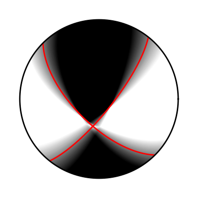
Fuzzy beachball illustrating the solutions uncertainty.

Beachballs views for cross-sections:

It is useful to show beachballs from other view angles, as in cross-sections. For that, we can define a view for all beachball plotting functions as shown here:

Download beachball_example06.py

import matplotlib.pyplot as plt
from pyrocko.plot import beachball, mpl_color
from pyrocko import moment_tensor as pmt


nrows = ncols = 3

fig = plt.figure(figsize=(6, 6))
axes = fig.add_subplot(1, 1, 1, aspect=1.)
fig.subplots_adjust(left=0., right=1., bottom=0., top=1.)
axes.axison = False
axes.set_xlim(-0.05 - ncols, ncols + 0.05)
axes.set_ylim(-0.05 - nrows, nrows + 0.05)

mt = pmt.as_mt((5., 90, 5.))

for view, irow, icol in [
        ('top', 1, 1),
        ((-90-45, 90.), 0, 0),
        ('north', 0, 1),
        ((-45, 90.), 0, 2),
        ('east', 1, 2),
        ((45., 90.), 2, 2),
        ('south', 2, 1),
        ((90.+45., 90.), 2, 0),
        ('west', 1, 0)]:

    beachball.plot_beachball_mpl(
        mt, axes,
        position=(icol*2-ncols+1, -irow*2+nrows-1),
        size_units='data',
        linewidth=1.0,
        color_t=mpl_color('skyblue2'),
        view=view)

    axes.annotate(
        view,
        xy=(icol*2-ncols+1, -irow*2+nrows-1.75),
        xycoords='data',
        xytext=(0, 0),
        textcoords='offset points',
        verticalalignment='center',
        horizontalalignment='center',
        rotation=0.)

fig.savefig('beachball_example06.png')
plt.show()

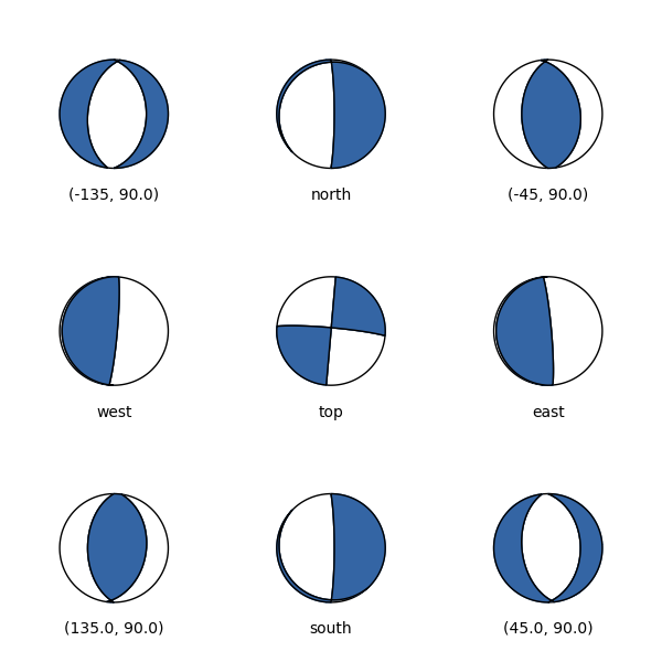
Beachball from top (center) and 8 different cross-sections.

Add station symbols to focal sphere diagram

This example shows how to add station symbols at the positions where P wave rays pierce the focal sphere.

The function to plot focal spheres (pyrocko.plot.beachball.plot_beachball_mpl()) uses the function pyrocko.plot.beachball.project() in the final projection from 3D to 2D coordinates. Here we use this function to place additional symbols on the plot. The take-off angles needed can be computed with some help of the pyrocko.cake module. Azimuth and distance computations are done with functions from pyrocko.orthodrome. Polarities are obtained with pyrocko.plot.beachball.amplitudes().

Download beachball_example04.py

import numpy as num
from matplotlib import pyplot as plt
from pyrocko import moment_tensor as pmt, cake, orthodrome
from pyrocko.plot import beachball

km = 1000.

# source position and mechanism
slat, slon, sdepth = 0., 0., 10.*km
mt = pmt.MomentTensor.random_dc()

# receiver positions
rdepth = 0.0
rlatlons = [
    (50., 10.),
    (60., -50.),
    (-30., 60.),
    (0.8, 0.8),  # first arrival is P  -> takeoff angle < 90deg
    (0.5, 0.5),  # first arrival is p  -> takeoff angle > 90deg
]

# earth model and phase for takeoff angle computations
mod = cake.load_model('ak135-f-continental.m')
phases = cake.PhaseDef.classic('P')

# setup figure with aspect=1.0/1.0, ranges=[-1.1, 1.1]
fig = plt.figure(figsize=(2., 2.))  # size in inch
fig.subplots_adjust(left=0., right=1., bottom=0., top=1.)
axes = fig.add_subplot(1, 1, 1, aspect=1.0)
axes.set_axis_off()
axes.set_xlim(-1.1, 1.1)
axes.set_ylim(-1.1, 1.1)

projection = 'lambert'

beachball.plot_beachball_mpl(
    mt, axes,
    position=(0., 0.),
    size=2.0,
    color_t=(0.7, 0.4, 0.4),
    projection=projection,
    size_units='data')

for rlat, rlon in rlatlons:
    distance = orthodrome.distance_accurate50m(slat, slon, rlat, rlon)
    rays = mod.arrivals(
        phases=[cake.PhaseDef('P'), cake.PhaseDef('p')],
        zstart=sdepth, zstop=rdepth, distances=[distance*cake.m2d])

    if not rays:
        continue

    takeoff = rays[0].takeoff_angle()
    azi = orthodrome.azimuth(slat, slon, rlat, rlon)
    polarity = num.sign(beachball.amplitudes(mt, [azi], [takeoff]))

    # to spherical coordinates, r, theta, phi in radians
    # flip direction when takeoff is upward
    rtp = num.array([[
        1.0 if takeoff <= 90. else -1.,
        num.deg2rad(takeoff),
        num.deg2rad(90.-azi)]])
    # to 3D coordinates (x, y, z)
    points = beachball.numpy_rtp2xyz(rtp)

    # project to 2D with same projection as used in beachball
    x, y = beachball.project(points, projection=projection).T

    axes.plot(
        x, y,
        '+' if polarity > 0.0 else 'x',
        ms=10. if polarity > 0.0 else 10./num.sqrt(2.),
        mew=2.0,
        mec='black',
        mfc='none')

fig.savefig('beachball-example04.png')

Focal sphere diagram with markers at positions of P wave ray piercing points.

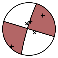
Hudson’s source type plot

Hudson’s source type plot [Hudson, 1989] is a way to visually represent the widely used “standard” decomposition of a moment tensor into its isotropic, its compensated linear vector dipole (CLVD), and its double-couple (DC) components.

The function pyrocko.plot.hudson.project() may be used to get the (u,v) coordinates for a given (full) moment tensor used for positioning the symbol in the plot. The function pyrocko.plot.hudson.draw_axes() can be used to conveniently draw the axes and annotations. Note, that we follow the original convention introduced by Hudson, to place the negative CLVD on the right hand side.

Download hudson_diagram.py

import sys
from matplotlib import pyplot as plt
from pyrocko.plot import hudson, beachball, mpl_init, mpl_color
from pyrocko import moment_tensor as pmt

# a bunch of random MTs
moment_tensors = [pmt.random_mt() for _ in range(200)]

# setup plot layout
fontsize = 10.
markersize = fontsize
mpl_init(fontsize=fontsize)
width = 7.
figsize = (width, width / (4. / 3.))
fig = plt.figure(figsize=figsize)
axes = fig.add_subplot(1, 1, 1)
fig.subplots_adjust(left=0.03, right=0.97, bottom=0.03, top=0.97)

# draw focal sphere diagrams for the random MTs
for mt in moment_tensors:
    u, v = hudson.project(mt)
    try:
        beachball.plot_beachball_mpl(
            mt, axes,
            beachball_type='full',
            position=(u, v),
            size=markersize,
            color_t=mpl_color('skyblue3'),
            color_p=mpl_color('skyblue1'),
            alpha=1.0,  # < 1 for transparency
            zorder=1,
            linewidth=0.25)

    except beachball.BeachballError as e:
        print(str(e), file=sys.stderr)

# draw the axes and annotations of the hudson plot
hudson.draw_axes(axes)

fig.savefig('hudson_diagram.png', dpi=150)
# plt.show()

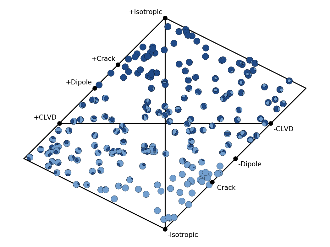
Hudson’s source type plot for 200 random moment tensors.

Source radiation plot

The directivity and radiation characteristics of any point or finite Source model can be illustrated with plot_directivity().

Radiation pattern effects

The following educational example illustrates radiation pattern effects from a point source in a homogeneous full space. Analytical Green’s functions for a homogeneous full space are computed within the example code by use of the ahfullgreen backend of Fomosto.

Download plot_directivity.py

import os
import shutil
from pyrocko.plot.directivity import plot_directivity
from pyrocko.gf import LocalEngine, DCSource, Store
from pyrocko.fomosto import ahfullgreen

km = 1e3


def make_homogeneous_gf_store(
        path, store_id, source_depth, receiver_depth, distance):

    if os.path.exists(path):
        shutil.rmtree(path)

    ahfullgreen.init(path, None, config_params=dict(
        id=store_id,
        sample_rate=20.,
        receiver_depth=receiver_depth,
        source_depth_min=source_depth,
        source_depth_max=source_depth,
        distance_min=distance,
        distance_max=distance))

    store = Store(path)
    store.make_travel_time_tables()
    ahfullgreen.build(path)


store_id = 'gf_homogeneous_radpat'
store_path = os.path.join('.', store_id)
distance = 10*km
receiver_depth = 0.0

source = DCSource(
    depth=0.,
    strike=0.,
    dip=90.,
    rake=0.)

make_homogeneous_gf_store(
    store_path, store_id, source.depth, receiver_depth, distance)

engine = LocalEngine(store_dirs=[store_path])

# import matplotlib.pyplot as plt
# fig = plt.figure(figsize=(7,5))
# axes = fig.add_subplot(111, polar=True)

resp = plot_directivity(
    engine, source, store_id,
    # axes=axes,
    distance=distance,
    dazi=5.,
    component='R',
    target_depth=receiver_depth,
    plot_mt='full',
    show_phases=True,
    fmin=None,
    fmax=1.0,
    phases={
        'P': '{stored:anyP}-50%',
        'S': '{stored:anyS}+50%'
    },
    interpolation='nearest_neighbor',
    quantity='velocity',
    envelope=False,
    hillshade=False)

# fig.savefig('radiation_pattern.png')

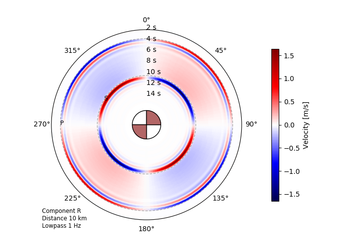
Radial component radiation pattern for a double-couple point source in a homogeneous full space observed in the plane of the source at a distance of 10 km. Note that the S waves seen in this example are pure near-field effects. They get less pronounced when going to higher frequencies.

Directivity effects

Synthetic seismic traces (R, T or Z) are forward-modelled at a defined radius, covering the full or partial azimuthal range and projected on a polar plot. Difference in the amplitude are enhanced by hillshading the data.

Download plot_directivity.py

import os
from pyrocko.plot.directivity import plot_directivity
from pyrocko.gf import LocalEngine, RectangularSource, ws

km = 1e3
# The store we are going extract data from:
store_id = 'iceland_reg_v2'

# First, download a Greens Functions store. If you already have one that you
# would like to use, you can skip this step and point the *store_superdirs* in
# the next step to that directory.

if not os.path.exists(store_id):
    ws.download_gf_store(site='kinherd', store_id=store_id)

# We need a pyrocko.gf.Engine object which provides us with the traces
# extracted from the store.
engine = LocalEngine(store_superdirs=['.'])

# Create a RectangularSource with uniform fit.
rect_source = RectangularSource(
    depth=1.6*km,
    strike=240.,
    dip=76.6,
    rake=-.4,
    anchor='top',
    nucleation_x=-.57,
    nucleation_y=-.59,
    velocity=2070.,
    length=27*km,
    width=9.4*km,
    slip=1.4)


# import matplotlib.pyplot as plt
# fig = plt.figure(figsize=(7,5))
# axes = fig.add_subplot(111, polar=True)

resp = plot_directivity(
    engine, rect_source, store_id,
    # axes=axes,
    distance=300*km,
    dazi=5.,
    component='R',
    plot_mt='full',
    show_phases=True,
    phases={
        'First': 'first{stored:begin}-10%',
        'Last': 'last{stored:end}+20'
    },
    quantity='displacement',
    envelope=False)

# fig.savefig('directivity_rectangular.png')

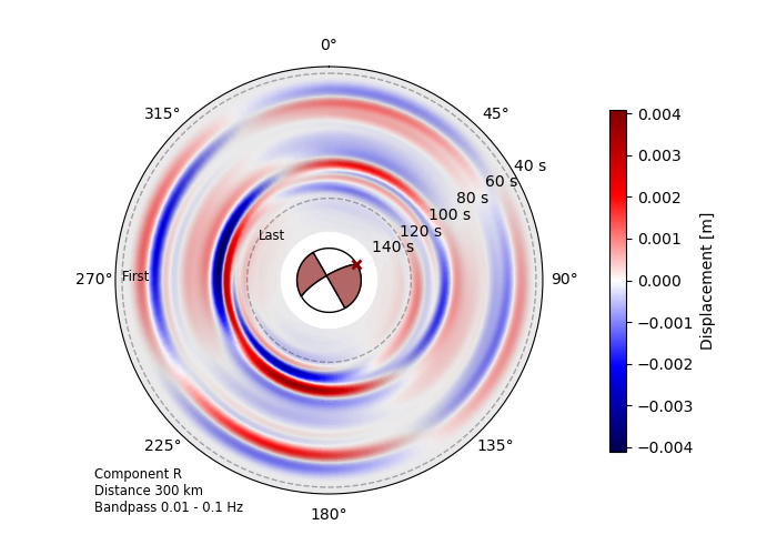
Source radiation pattern at 300 km distance of the Mw 6.8 2020 Elazig-Sevrice earthquake. The dominantly unilateral strike-slip rupture is reconstructed by a finite RectangularSource model.

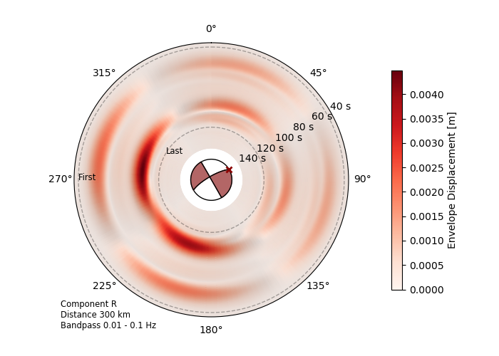
Here we see the envelope of the synthetic seismic traces, emphasizing the directivity effects of the source (envelope=True). Same source model: Mw 6.8 2020 Elazig-Sevrice earthquake.

Pseudo dynamic rupture - slip map, slip movie, source plots

The different attributes, rupture dislocations and their evolution over time of the PseudoDynamicRupture can be inspected and illustrated in different ways from map view to small gifs. The illustration of patch wise attributes is also possible with the built-in module dynamic_rupture.

Maps of the given patch attributes or the rupture dislocation at any time can be displayed using RuptureMap.

Download dynamic_rupture_map.py

import os

from pyrocko import gf
from pyrocko.gf import tractions, ws, LocalEngine
from pyrocko.plot import dynamic_rupture


# The store we are going extract data from:
store_id = 'iceland_reg_v2'

# First, download a Greens Functions store. If you already have one that you
# would like to use, you can skip this step and point the *store_superdirs* in
# the next step to that directory.

if not os.path.exists(store_id):
    ws.download_gf_store(site='kinherd', store_id=store_id)

# We need a pyrocko.gf.Engine object which provides us with the traces
# extracted from the store. In this case we are going to use a local
# engine since we are going to query a local store.
engine = LocalEngine(store_superdirs=['.'], default_store_id=store_id)

# The dynamic parameter used for discretization of the PseudoDynamicRupture are
# extracted from the stores config file.
store = engine.get_store(store_id)

# Define the traction structure as a composition of a homogeneous traction and
# a rectangular taper tapering the traction at the edges of the rupture
tracts = tractions.TractionComposition(
    components=[
        tractions.HomogeneousTractions(
            strike=1.e6,
            dip=0.,
            normal=0.),
        tractions.RectangularTaper()])

# Let's define the source now with its extension, orientation etc.
source = gf.PseudoDynamicRupture(
    lat=6.45,
    lon=37.06,
    length=30000.,
    width=10000.,
    strike=215.,
    dip=45.,
    anchor='top',
    gamma=0.6,
    depth=2000.,
    nucleation_x=0.25,
    nucleation_y=-0.5,
    nx=20,
    ny=10,
    pure_shear=True,
    tractions=tracts)

# The define PseudoDynamicSource needs to be divided into finite fault elements
# which is done using spacings defined by the greens function data base
source.discretize_patches(store)

# Define the rupture map object parameters as image center coordinates,
# radius in m and the size of the image
map_kwargs = dict(
    lat=6.50,
    lon=37.06,
    radius=20000.,
    width=25.,
    height=25.,
    source=source,
    show_topo=True)

# Initialize the map with the set arguments and display the traction vector
# length per patch.
m = dynamic_rupture.RuptureMap(**map_kwargs)
m.draw_patch_parameter('traction', cbar=True, anchor='top_right')
m.draw_nucleation_point()
m.save('traction_map.png')

# Initialize the map and generate a more complex plot of the dislocation at
# 3 s after origin time with the corresponding dislocation contour lines with
# a contour line at 0.15 m total dislocation. Also the belonging rupture front
# contour at 3 s is displayed together with nucleation point.
m = dynamic_rupture.RuptureMap(**map_kwargs)
m.draw_dislocation(time=3, cmap='summer')
# dislocation vector drawing needs update as it triggers an error on newer
# GMTs:
# m.draw_dislocation_vector(time=3, S='i5p', I='x20')
m.draw_time_contour(store, clevel=[3])
m.draw_dislocation_contour(time=3, clevel=[0.15])
m.draw_nucleation_point()
m.save('dislocation_map_3s.png')

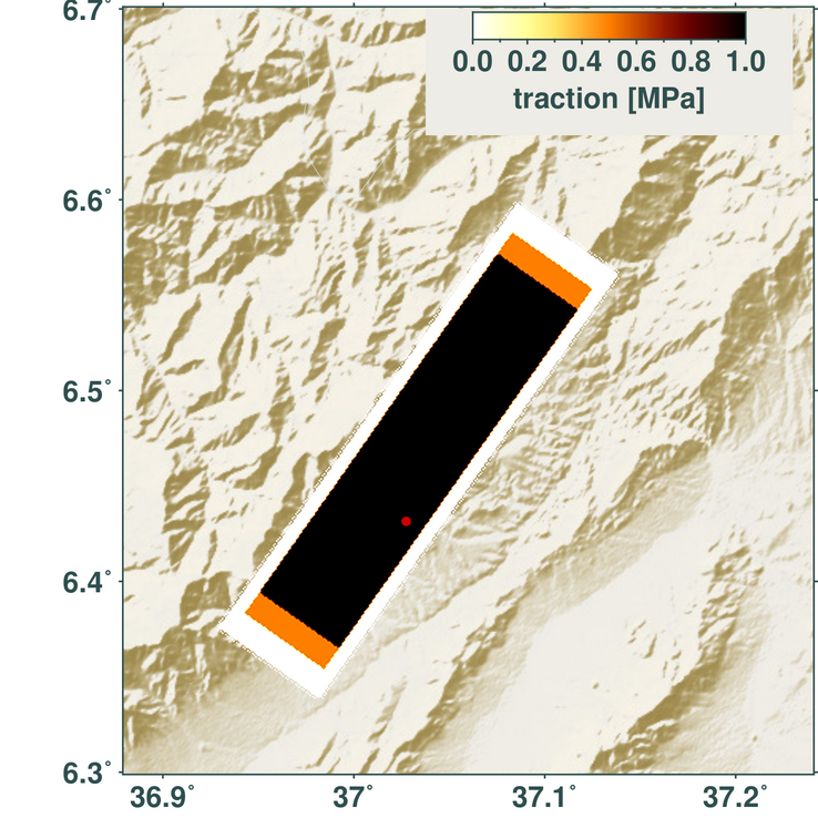
Length of the stress drop vectors, which act on each subfault (patch) of the PseudoDynamicRupture.

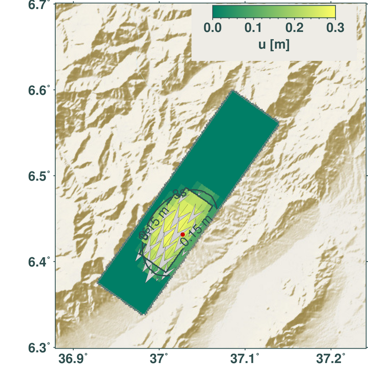
Shown is the length of the dislocation vectors of each subfault 3 s after the rupture initiation. The rupture nucleation point is marked with the red dot, the contour line indicates the tip of the rupture front. Arrows show the length and direction of the slip vectors on the plane (shear only).

On plane views of the given patch attributes or the rupture dislocation at any time can be displayed using RuptureView. It also allows to inspect single patch time lines as slip, slip rate or moment rate.

Download dynamic_rupture_viewer.py

import os

from pyrocko import gf
from pyrocko.gf import tractions, ws, LocalEngine
from pyrocko.plot import dynamic_rupture


# The store we are going extract data from:
store_id = 'iceland_reg_v2'

# First, download a Greens Functions store. If you already have one that you
# would like to use, you can skip this step and point the *store_superdirs* in
# the next step to that directory.

if not os.path.exists(store_id):
    ws.download_gf_store(site='kinherd', store_id=store_id)

# We need a pyrocko.gf.Engine object which provides us with the traces
# extracted from the store. In this case we are going to use a local
# engine since we are going to query a local store.
engine = LocalEngine(store_superdirs=['.'], default_store_id=store_id)

# The dynamic parameter used for discretization of the PseudoDynamicRupture are
# extracted from the stores config file.
store = engine.get_store(store_id)

# Define the traction structure as a composition of a homogeneous traction and
# a rectangular taper tapering the traction at the edges of the rupture
tracts = tractions.TractionComposition(
    components=[
        tractions.HomogeneousTractions(
            strike=1.e6,
            dip=0.,
            normal=0.),
        tractions.RectangularTaper()])

# Let's define the source now with its extension, orientation etc.
source = gf.PseudoDynamicRupture(
    lat=-21.,
    lon=32.,
    length=30000.,
    width=10000.,
    strike=165.,
    dip=45.,
    anchor='top',
    gamma=0.6,
    depth=2000.,
    nucleation_x=0.25,
    nucleation_y=-0.5,
    nx=20,
    ny=10,
    pure_shear=True,
    tractions=tracts)

# The define PseudoDynamicSource needs to be divided into finite fault elements
# which is done using spacings defined by the greens function data base
source.discretize_patches(store)

# Initialize the viewer and display the seismic moment release of the source
# over time with a sampling interval of 1 s
viewer = dynamic_rupture.RuptureView(source=source)
viewer.draw_source_dynamics(variable='moment', deltat=1, store=store)
viewer.save('dynamic_view_source_moment.png')
viewer.show_plot()

# Initialize the viewer and display the seismic moment release of one single
# boundary element (patch) over time
viewer = dynamic_rupture.RuptureView(source=source)
viewer.draw_patch_dynamics(variable='moment', nx=3, ny=3, deltat=1)
viewer.save('dynamic_view_patch_moment.png')
viewer.show_plot()

# Initialize the viewer and display the traction vector length.
viewer.draw_patch_parameter('traction')
viewer.draw_nucleation_point()
viewer.save('dynamic_view_source_traction.png')
viewer.show_plot()

# Initialize the viewer and generate a more complex plot of the dislocation at
# 3 s after origin time with the corresponding dislocation contour lines with
# a contour line at 0.15 m total dislocation. Also the belonging rupture front
# contour at 3 s is displayed together with nucleation point.
viewer.draw_dislocation(time=3, cmap='summer')
viewer.draw_time_contour(store, clevel=[3])
viewer.draw_dislocation_contour(time=3, clevel=[0.15])
viewer.draw_nucleation_point()
viewer.save('dynamic_view_source_dislocation.png')
viewer.show_plot()

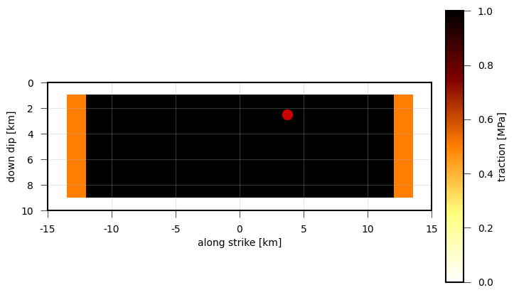
Length of the stress drop vectors, which act on each subfault (patch) of the PseudoDynamicRupture.

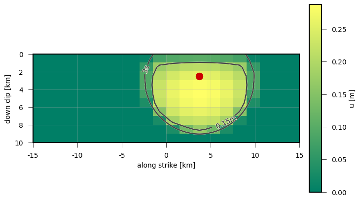
Shown is the length of the dislocation vectors of each subfault 3 s after the rupture initiation. The rupture nucleation point is marked with the red dot, the contour line indicates the tip of the rupture front.

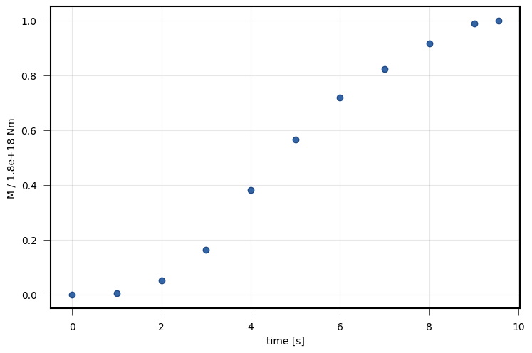
Shown is the sum of all subfault seismic moment releases of the PseudoDynamicRupture.

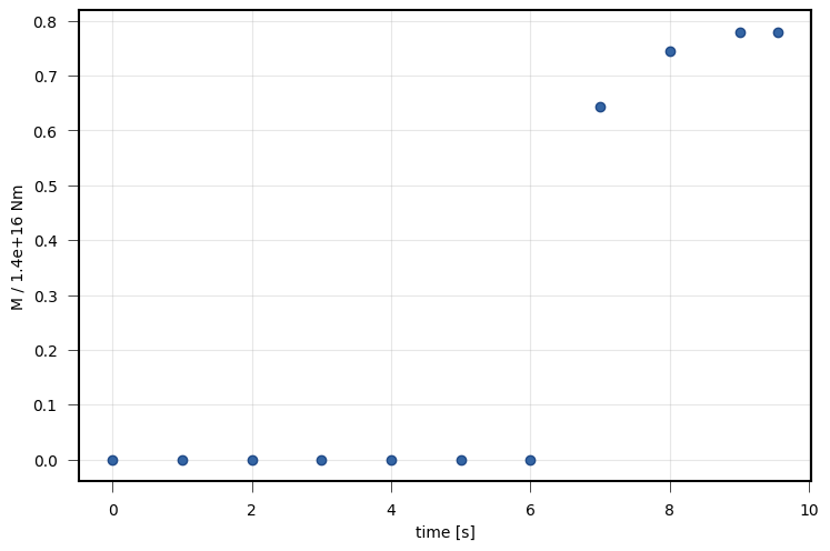
Each patch has an individual time dependent moment release function. Here the cumulative seismic moment over time is shown for the patch at 4th position along strike and 4th position down dip.