
Centroid moment tensor from regional surface wave observations
This step-by-step guide explains how to obtain a probabilistic centroid moment tensor (CMT) solution from surface waves for an Mw 5.9 aftershock of the Mw 6.9 2018 Indonesia earthquake using Grond.
Setup
To repeat this exercise on your machine, you should first install Pyrocko and Grond (see Installation), if you have not already done so. Then create the example project with:
grond init example_regional_cmt grond-playground-regional/
The project folder
The project folder now contains a configuration file for Grond, some utility scripts to download pre-calculated Green’s functions and to download seismic waveforms from public data centres.
grond-playground-regional  # project folder
├── bin                         # directory with scripts
│   ├── download_gf_stores.sh   # download pre-calculated Green's functions
│   ├── grondown                # a simple event-based waveform downloader
│   └── grondown_regional.sh    # downloader configured for this exercise
└── config                      # directory for configuration files
    └── surface_cmt.gronf       # Grond configuration file for this exercise
Green’s function download
To download the pre-calculated Green’s functions needed in this exercise, run
bin/download_gf_stores.sh
When the command succeeds, you should have a new subdirectory gf_stores in your project folder:
gf_stores
└── crust2_j3/... # Green's function store
It contains a Pyrocko Green’s function store, named crust2_j3, which has been created using the Fomosto tool of Pyrocko and the modelling code QSEIS. The Green’s functions in this store have been calculated for a regional Crust2x2 earth model for a source depths between 0 and 30 km in 1 km steps. It is sampled at 2 Hz, which is sufficient for our target frequency range of 0.01 - 0.1 Hz.
Seismic waveform data download
A preconfigured script is provided to download seismic waveform recordings via FDSN web services from the IRIS and GEOFON data centers. Just run it with the GEOFON event ID of the study earthquake. The GEOFON event ID of the Mw 5.9 aftershock is gfz2018pmjk (you can find the ID in the GEOFON catalog event links).
To download the seismic waveform data, now run:
bin/grondown_regional.sh gfz2018pmjk
This shell script calls the data downloader bin/grondown with parameters appropriate to get a dataset of broadband seismometer recordings, sufficient for a surface wave CMT optimisation. It performs the following steps for us:
Query the GEOFON catalog for event information about
gfz2018pmjk.Select time windows based on event origin and time, considering that we want to analyse the signals at low frequencies (0.01 - 0.1 Hz).
Query data centres for seismic stations with epicentral distance between 0 and 1000 km.
From the available recorder channels select appropriate ones for a target sampling rate of 2 Hz.
Download raw waveform data for the selected stations and channels.
Download instrument transfer function meta-information for all successfully downloaded waveform data.
Calculate displacement seismograms for quality check (Grond will use the raw data). If all went well, the displacement seismograms should be valid in the frequency range 0.01 - 0.05 Hz, sampled at 1 Hz and rotated to radial, transverse, and vertical components. The rotation to radial and transverse components is with respect to the event coordinates from the GEOFON catalogue.
After running the download script, the playground directory should contain a new data directory with the following content:
data
└── events
    └── gfz2018pmjk
        ├── event.txt                 # catalogue information about the event
        └── waveforms
            ├── grondown.command
            ├── prepared/...          # rotated, displacement waveforms
            ├── raw/...               # raw Mini-SEED waveforms
            ├── rest/...
            ├── stations.geofon.xml   # instrument response information
            ├── stations.iris.xml
            ├── stations.orfeus.xml
            ├── stations.prepared.txt # stations files for Snuffler
            └── stations.raw.txt
Because of various data problems, like missing instrument response information, gappy traces, data inconsistencies and what not, only about half of the initially requested stations will be useful in the optimisation. Some problems are not detected by the downloader, so we will have to look at the seismograms.
Data screening
For a quick visual inspection of the dataset, we can use the Snuffler program contained in Pyrocko.
cd data/events/gfz2018pmjk/waveforms
snuffler --event=../event.txt --stations=stations.prepared.txt prepared
cd -  # change to previous folder
Figure 1 shows our view after some interactive adjustments in Snuffler. In particular, we may want to
sort the traces according to epicentral distance (Menu → check Sort by Distance).
configure display style (Menu → uncheck Show Boxes, check Common Scale per Station, uncheck Clip Traces).
filter between 0.01 and 0.05 Hz.
add markers for expected P phase arrivals, (Menu → Panels → Cake Phase (builtin)).
show only vertical components: Command ‣ c *z.

Figure 1: Displacement seismograms for surface wave CMT optimisation as viewed in the waveform browser Snuffler.
Grond configuration
The project folder already contains a configuration file for W-phase CMT optimisation with Grond, so let’s have a look at it. It is a YAML file. If you have never heard about this file format, read section Configuration file structure and format (YAML) for an overview.
%YAML 1.1
# Example: Inversion of centroid moment tensor from regional waveform observations.
--- !grond.Config

# All file paths referenced below are treated relative to the location of this
# configuration file, here we may give a common prefix. E.g. setting it to '..'
# if the configuration file is in the sub-directory '${project_root}/config'
# allows us to give the paths below relative to '${project_root}'.
path_prefix: '..'

# Path, where to store output (run directories). The placeholder
# '${problem_name}' will be expanded to a name configured below in
# problem_config.name_template and will typically include a config identifier
# and the event name.
rundir_template: 'runs/${problem_name}.grun'

# If given, restrict to processing of listed events
#event_names:
#- 'gfz2018pmjk'


# -----------------------------------------------------------------------------
# Configuration section for dataset (input data)
#
# The placeholder '${event_name}' will be expanded to the current event. This
# enables us to use the same configuration for multiple events. The available
# events are detected by looking into possible expansions of
# dataset_config.events_path
# -----------------------------------------------------------------------------

dataset_config: !grond.DatasetConfig
  # More information on the data configuration at
  # https://pyrocko.org/grond/docs/current/config/dataset/index.html

  # List of files with station coordinates.
  stations_stationxml_paths:
  - 'data/events/${event_name}/waveforms/stations.geofon.xml'
  - 'data/events/${event_name}/waveforms/stations.iris.xml'

  # File with hypocenter information and possibly reference solution
  events_path: 'data/events/${event_name}/event.txt'

  # List of directories with raw waveform data
  waveform_paths: ['data/events/${event_name}/waveforms/raw']

  # List of stations/components to be excluded according to their STA, NET.STA,
  # NET.STA.LOC, or NET.STA.LOC.CHA codes
  exclude: ['GE.UGM', 'GE.PLAI']

  # List of files with additional exclusion lists (one entry per line, same
  # format as above)
  exclude_paths:
  - 'data/events/${event_name}/waveforms/exclude.txt'

  # List of files with instrument response information (can be the same as in
  # stations_stationxml_paths above)
  responses_stationxml_paths:
  - 'data/events/${event_name}/waveforms/stations.geofon.xml'
  - 'data/events/${event_name}/waveforms/stations.iris.xml'

  # Apply correction factors from station corrections.
  apply_correction_factors: true

  # Extend incomplete seismic traces
  extend_incomplete: false

# -----------------------------------------------------------------------------
# Configuration section for the observational data fitting
#
# This defines the objective function to be minimized in the optimisation. It
# can be composed of one or more contributions, each represented by a
# !grond.*TargetGroup section.
# -----------------------------------------------------------------------------

target_groups:
- !grond.WaveformTargetGroup

  # Normalisation family (see the Grond documentation for how it works).
  # Use distinct normalisation families when mixing misfit contributors with
  # different magnitude scaling, like e.g. cross-correlation based misfit and
  # time-domain Lx norm.
  normalisation_family: 'td'

  # Just a name used to identify targets from this group. Use dot-separated path
  # notation to group related contributors
  path: 'td.love'

  # Epicentral distance range of stations to be considered in meter
  distance_min: 1e3
  distance_max: 900e3

  # Names of components to be included. Available: N=north, E=east, Z=vertical
  # (up), R=radial (away), T=transverse (right)
  channels: ['T']

  # How to weight contributions from this group in the global misfit
  weight: 1.0

  # subsection on how to fit the traces
  misfit_config: !grond.WaveformMisfitConfig

    # Frequency band [Hz] of acausal filter (flat part of frequency taper)
    fmin: 0.01
    fmax: 0.05

    # Factor defining fall-off of frequency taper (zero at fmin/ffactor and
    # fmax*ffactor)
    ffactor: 1.5

    # Time window to include in the data fitting. Times can be defined offset
    # to given phase arrivals. E.g. '{stored:P}-600' would mean 600 s
    # before arrival of the phase named 'P'. The phase must be defined in the
    # travel time tables in the GF store.
    tmin: '{stored:any_P}'
    tmax: '{vel_surface:2.5}'
    # tfade: 120.0

    # How to fit the data (available: 'time_domain', 'frequency_domain',
    # 'log_frequency_domain', 'absolute', 'envelope', 'cc_max_norm')
    domain: 'time_domain'

    # If non-zero, allow synthetic and observed traces to be shifted
    # against each other by up to +/- the given value [s].
    tautoshift_max: 4.0

    # If non-zero, a penalty misfit is added for non-zero shift values.
    # The penalty value is computed as
    # autoshift_penalty_max * normalization_factor * tautoshift**2 / tautoshift_max**2
    autoshift_penalty_max: 0.05

    # For L1 norm: 1, L2 norm: 2, etc.
    norm_exponent: 1

  # How to interpolate the Green's functions (available choices:
  # 'nearest_neighbor', 'multilinear'). Choices other than 'nearest_neighbor'
  # may require dense GF stores to avoid aliasing artifacts in the forward
  # modelling.
  interpolation: 'nearest_neighbor'

  # Name of the GF Store to use
  store_id: 'crust2_j3'

  # Instead of defining a GF store, the Crust2StoreIDSelector can be used
  # to automatically pick the CRUST 2.0 model based on the event location.
  # store_id_selector: !grond.Crust2StoreIDSelector
  #   template: crust2_${id}


- !grond.WaveformTargetGroup

  # Normalisation family (see the Grond documentation for how it works).
  # Use distinct normalisation families when mixing misfit contributors with
  # different magnitude scaling, like e.g. cross-correlation based misfit and
  # time-domain Lx norm.
  normalisation_family: 'td'

  # Just a name used to identfy targets from this group. Use dot-separated path
  # notation to group related contributors
  path: 'td.rayleigh'

  # Epicentral distance range of stations to be considered in meter
  distance_min: 1e3
  distance_max: 900e3

  # Names of components to be included. Available: N=north, E=east, Z=vertical
  # (up), R=radial (away), T=transverse (right)
  channels: ['R', 'Z']

  # How to weight contributions from this group in the global misfit
  weight: 1.0

  # subsection on how to fit the traces
  misfit_config: !grond.WaveformMisfitConfig

    # Frequency band [Hz] of acausal filter (flat part of frequency taper)
    fmin: 0.01
    fmax: 0.05

    # Factor defining fall-off of frequency taper (zero at fmin/ffactor and
    # fmax*ffactor)
    ffactor: 1.5

    # Time window to include in the data fitting. Times can be defined offset
    # to given phase arrivals. E.g. '{stored:P}-600' would mean 600 s
    # before arrival of the phase named 'P'. The phase must be defined in the
    # travel time tables in the GF store.
    tmin: '{stored:any_P}'
    tmax: '{vel_surface:2.5}'
    # tfade: 120.0

    # How to fit the data (available: 'time_domain', 'frequency_domain',
    # 'log_frequency_domain', 'absolute', 'envelope', 'cc_max_norm')
    domain: 'time_domain'

    # If non-zero, allow synthetic and observed traces to be shifted
    # against each other by up to +/- the given value [s].
    tautoshift_max: 4.0

    # If non-zero, a penalty misfit is added for non-zero shift values.
    # The penalty value is computed as
    # autoshift_penalty_max * normalization_factor * tautoshift**2 / tautoshift_max**2
    autoshift_penalty_max: 0.05

    # For L1 norm: 1, L2 norm: 2, etc.
    norm_exponent: 1

  # How to interpolate the Green's functions (available choices:
  # 'nearest_neighbor', 'multilinear'). Choices other than 'nearest_neighbor'
  # may require dense GF stores to avoid aliasing artifacts in the forward
  # modelling.
  interpolation: 'nearest_neighbor'

  # Name of the GF Store to use
  store_id: 'crust2_j3'


# -----------------------------------------------------------------------------
# Definition of the problem to be solved
#
# In this section the source model to be fitted is chosen, the parameter space
# defined, and how to combine the misfit contributions defined in the
# target_groups section above.
#
# The marker !grond.CMTProblemConfig selects a centroid moment tensor source
# model.
# -----------------------------------------------------------------------------
problem_config: !grond.CMTProblemConfig

  # Name used to identify the output
  name_template: 'cmt_${event_name}'

  # Definition of model parameter space to be searched in the optimisation
  ranges:
    # Time relative to hypocenter origin time [s]
    time: '-10 .. 10 | add'

    # Centroid location with respect to hypocenter origin [m]
    north_shift: '-15e3 .. 15e3'
    east_shift: '-15e3 .. 15e3'
    depth: '5e3 .. 30e3'

    # Range of magnitudes to allow
    magnitude: '5.7 .. 6.2'

    # Relative moment tensor component ranges (don't touch)
    rmnn: '-1.41421 .. 1.41421'
    rmee: '-1.41421 .. 1.41421'
    rmdd: '-1.41421 .. 1.41421'
    rmne: '-1 .. 1'
    rmnd: '-1 .. 1'
    rmed: '-1 .. 1'

    # Source duration range [s]
    duration: '1. .. 5.'

  # Clearance distance around stations (no models with origin closer than this
  # distance to any station are produced by the sampler)
  distance_min: 1e3

  # Type of moment tensor to restrict to (choices: 'full', 'deviatoric', 'dc')
  mt_type: 'deviatoric'

  # How to combine the target misfits. For L1 norm: 1, L2 norm: 2, etc.
  norm_exponent: 1


# -----------------------------------------------------------------------------
# Configuration of pre-optimisation analysis phases.
# determined during this phase.
# -----------------------------------------------------------------------------
#
analyser_configs:

# Balancing weights are determined with this analyser
- !grond.TargetBalancingAnalyserConfig

  # Number of models to forward model in the analysis, larger number -> better
  # statistics)
  niterations: 1000

# -----------------------------------------------------------------------------
# Configuration of the optimisation procedure
# -----------------------------------------------------------------------------
optimiser_config: !grond.HighScoreOptimiserConfig

  # Number of bootstrap realisations to be tracked simultaneously in the
  # optimisation
  nbootstrap: 100

  # stages of the sampler. Start with uniform sampling of the model space
  # (!grond.UniformSamplerPhase), then narrow down to the interesting regions
  # (!grond.DirectedSamplerPhase).
  sampler_phases:

  - !grond.UniformSamplerPhase
      # Number of iterations
      niterations: 1000

  - !grond.DirectedSamplerPhase
      # Number of iterations
      niterations: 20000

      # Multiplicator for width of sampler distribution at start of this phase
      scatter_scale_begin: 2.0

      # Multiplicator for width of sampler distribution at end of this phase
      scatter_scale_end: 0.5


# -----------------------------------------------------------------------------
# Configuration section for synthetic seismogram engine
#
# Configures where to look for GF stores.
# -----------------------------------------------------------------------------

engine_config: !grond.EngineConfig

  # Whether to use GF store directories listed in ~/.pyrocko/config.pf
  gf_stores_from_pyrocko_config: false

  # List of directories with GF stores
  gf_store_superdirs: ['gf_stores']
Configured like this, Grond will try to fit Rayleigh waves in the frequency range 0.01 to 0.05 Hz on the vertical (Z) and radial (R) components as well as Love waves on the transverse (T) component of ground displacement. The mismatch between observation and modelling will be measured using an L1 norm.
Checking the optimisation setup
Before running the actual optimisation, we can now use the command
grond check config/regional_cmt.gronf gfz2018pmjk
to run some sanity checks. In particular, Grond will compare the configuration with the extent of the GF store, checking that the distance ranges and frequency ranges of the targets, and the depth range of the inversion problem are consistent with the GF store extent and sampling rate.
Next, grond check will try to run a few forward models to see if the modelling works and if it can read the input data. If only one event is available, we can also neglect the event name argument in this and other Grond commands.
To get some more insight into the setup, we can run
grond report -so config/regional_cmt.gronf gfz2018pmjk
This will plot some diagnostic figures, create web pages in a new directory report, and finally open these in a web browser.
Starting the optimisation
Let’s start the optimisation with:
grond go config/regional_cmt.gronf
During the optimisation a status monitor will show the optimisation’s progress.
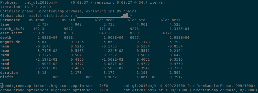
Depending on the configured number of iterations and the computer’s hardware the optimisation will run several minutes to hours.
Optimisation report
Once the optimisation is finished we can generate and open the final report with:
grond report -so runs/cmt_gfz2018pmjk.grun
Example report
Explore the online example reports to see what information the inversion reveals.