
Rectangular source plane from InSAR observations
This step-by-step recipe will guide you to through an earthquake source inversion for a finite rectangular fault plane from InSAR data using Grond. We will exercise the inversion for the 2009 L’Aquila earthquake - A shallow normal faulting Mw 6.3 earthquake - and use unwrapped surface displacement data derived from the Envisat mission.
Setup
To repeat this exercise on your machine, you should first install Pyrocko and Grond (see Installation), if you have not already done so. Then create the example project with:
grond init example_insar grond-playground-insar/
The project folder
The project folder now contains a configuration file for Grond and some utility scripts to download pre-calculated static Green’s functions and InSAR data:
grond-playground-insar        # project folder
├── bin                        # directory with scripts
│   ├── download_gf_stores.sh  # download pre-calculated Green's functions
│   ├── download_insar_data.sh      # a simple event-based waveform downloader
└── config                     # directory for configuration files
    └── insar_rectangular.gronf       # Grond configuration file for this exercise
Green’s function download
To download the pre-calculated Green’s functions needed in this exercise, run
bin/download_gf_stores.sh
When the command succeeds, you should have a new subdirectory gf_stores in your project folder:
gf_stores
└── crust2_ib_static/... # Green's function store
It contains a Pyrocko Green’s function store, named crust2_ib_static, which has been created using the Fomosto tool of Pyrocko and the modelling code PSGRN/PSCMP. The Green’s functions in this store have been calculated for a regional CRUST2 earth model for source depths between 0 and 30 km in 500 m steps, and horizontal extent from 0 - 300 km in 500 m steps.
InSAR displacement download
The example includes a script to download unwrapped InSAR data from Pyrocko’s servers. The surface displacement data has been derived from the Envisat satellite mission.
bin/download_insar_data.sh
This will download (1) an ascending and (2) descending scene to data/events/2009laquila/insar/. Data is held in Kite container format.
Unwrapped InSAR displacement preparation with Kite
The downloaded data has to be prepared for the inversion with the Kite tool. To install the software, follow the install instructions.
Once the software is installed we need to parametrize the two scenes:
The data sub-sampling quadtree: This efficiently reduces the resolution of the scene, yet conserves the important data information. A reduced number of samples will benefit the forward-modelling computing cost.
Estimate the spatial data covariance: By looking at the spatial noise of the scene we can estimate the data covariance. Kite enables us to calculate a covariance matrix for the quadtree, which will be used as a weight matrix in our Grond inversion.
We start by parametrizing the quadtree: find a good parameters for the sub-sampling quadtree by tuning four parameters:
epsilon, the variance threshold in each quadtree’s tile.
nan_fraction, percentage of allowed NaN pixels per tile.
tile_size_min, minimum size of the tiles.
tile_size_max, maximum size of the tiles.
Start Kite’s spool GUI with:
spool data/events/2009laquila/insar/asc_insar
# descending scene:
spool data/events/2009laquila/insar/dsc_insar
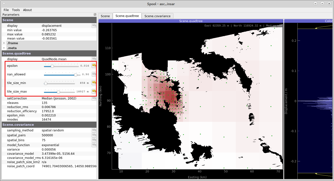
Figure 1: Parametrizing the quadtree. This efficiently sub-samples the high-resolution surface displacement data. (command spool; Kite toolbox).
Note
Delete unnecessary tiles of the quadtree by right-clicking, and delete with Del.
Once you are happy with the sub-sampling, click on the next tab Scene.covariance. Now we will define a window for the data’s noise. The window’s data will be use for calculating the spatial covariance of the scene (see details).
Use a spatial window far away from the earthquake signal to capture only the noise, yet the bigger the window is, the better the data covariance estimation.
On the left hand side of the GUI you find parameters to tune the spatial covariance analysis. We now can fit an analytical model to the empirical covariance: \(\exp(d)\) and \(\exp + \sin\). For more details on the method, see Kite’s documentation.
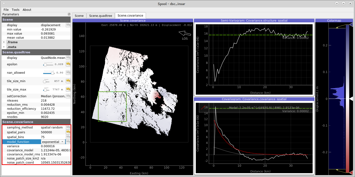
Figure 2: Data covariance inspection with spool.
Once we finished parametrisation of the quadtree and covariance, we have to calculate the full covariance and weight matrix from the complete scene resolution:
Calculate the full covariance:
Save the parametrized scene: .
Grond configuration
The project folder already contains a configuration file for rectangular source optimisation with Grond, so let’s have a look at it.
It’s a YAML file: This file format has been chosen for the Grond configuration because it can represent arbitrarily nested data structures built from mappings, lists, and scalar values. It also provides an excellent balance between human and machine readability. When working with YAML files, it is good to know that the indentation is part of the syntax and that comments can be introduced with the # symbol. The type markers, like !grond.RectangularProblemConfig, select the Grond object type of the following mapping and it’s documentation can likely be found in the Library reference.
%YAML 1.1
# Example: Inversion of planar rectangular source model from InSAR observations.
--- !grond.Config

# All file paths referenced below are treated relative to the location of this
# configuration file, here we may give a common prefix. E.g. setting it to '..'
# if the configuration file is in the sub-directory '${project_root}/config'
# allows us to give the paths below relative to '${project_root}'.
path_prefix: '..'

# Path, where to store output (run directories). The placeholder
# '${problem_name}' will be expanded to a name configured below in
# problem_config.name_template and will typically include a config identifier
# and the event name.
rundir_template: runs/${problem_name}.grun

# If given, restrict to processing of listed events
#event_names:
#- 'gfz2018pmjk'


# -----------------------------------------------------------------------------
# Configuration section for dataset (input data)
#
# The placeholder '${event_name}' will be expanded to the current event. This
# enables us to use the same configuration for multiple events. The available
# events are detected by looking into possible expansions of
# dataset_config.events_path
# -----------------------------------------------------------------------------

dataset_config: !grond.DatasetConfig

  # File with hypocenter information and possibly reference solution
  events_path: 'data/events/${event_name}/event.txt'

  # List of directories for the InSAR scenes
  kite_scene_paths: ['data/events/${event_name}/insar']

# -----------------------------------------------------------------------------
# Configuration section for the observational data fitting
#
# This defines the objective function to be minimized in the optimisation. It
# can be composed of one or more contributions, each represented by a
# !grond.*TargetGroup section.
# -----------------------------------------------------------------------------

target_groups:
- !grond.SatelliteTargetGroup

  # Normalisation family (see the Grond documentation for how it works).
  # Use distinct normalisation families when mixing misfit contributors with
  # different magnitude scaling, like e.g. cross-correlation based misfit and
  # time-domain Lx norm.
  normalisation_family: 'static'

  # Just a name used to identify targets from this group. Use dot-separated path
  # notation to group related contributors
  path: 'insar'

  # How to weight contributions from this group in the global misfit
  weight: 1.0

  # Selector for kite scene ids, '*all' is a wildcard and load all scenes present
  kite_scenes: ['*all']

  # Subsection on how to fit the traces
  misfit_config: !grond.SatelliteMisfitConfig

    # Optimise a planar orbital ramp
    optimise_orbital_ramp: false

    # Parameters for the orbital ramp
    ranges:

      # Vertical offset in [m]
      offset: -0.5 .. 0.5

      # Ranges for the East-West and North-South inclination of the ramp
      ramp_east: -1e-4 .. 1e-4
      ramp_north: -1e-4 .. 1e-4

  # How to interpolate the Green's functions (available choices:
  # 'nearest_neighbor', 'multilinear'). Choices other than 'nearest_neighbor'
  # may require dense GF stores to avoid aliasing artifacts in the forward
  # modelling.
  interpolation: multilinear

  # Name of the GF Store to use
  store_id: crust2_ib_static


# -----------------------------------------------------------------------------
# Definition of the problem to be solved
#
# In this section the source model to be fitted is chosen, the parameter space
# defined, and how to combine the misfit contributions defined in the
# target_groups section above.
#
# The marker !grond.RectangularProblemConfig selects a finite rectancular
# source model.
# -----------------------------------------------------------------------------
problem_config: !grond.RectangularProblemConfig

  # Name used to identify the output
  name_template: rect_2009LaAquila

  # How to combine the target misfits. For L1 norm: 1, L2 norm: 2, etc.
  norm_exponent: 2

  # Definition of model parameter space to be searched in the optimisation
  ranges:

    # Scaling ranges in [m]
    depth: 2500 .. 7000
    east_shift: 0 .. 20000
    north_shift: 0 .. 20000
    length: 5000 .. 10000
    width: 2000 .. 10000
    slip: .2 .. 2

    # Orientation ranges in [deg]
    dip: 10 .. 50
    rake: 120 .. 360
    strike: 220 .. 360

  # The number of subsources used in the modelling is dependent on the spatial
  # spacing of the Green's function in the GF Store. The decimation_factor
  # parameter allows to decrease the resolution of the discretised source model
  # (use fewer sub-sources) for speedy computation with inaccurate results (for
  # testing purposes). Higher value means faster computation and less accurate
  # result.
  decimation_factor: 1

  # Clearance distance around stations (no models with origin closer than this
  # distance to any station are produced by the sampler)
  distance_min: 0.0

# -----------------------------------------------------------------------------
# Configuration of pre-optimisation analysis phases.
# determined during this phase.
# -----------------------------------------------------------------------------
#
analyser_configs:

# DOES NOT APPLY FOR INSAR! Balancing weights are determined with this analyser
- !grond.TargetBalancingAnalyserConfig
  niterations: 1000

# -----------------------------------------------------------------------------
# Configuration of the optimisation procedure
# -----------------------------------------------------------------------------
optimiser_config: !grond.HighScoreOptimiserConfig
  # Number of bootstrap realisations to be tracked simultaneously in the
  # optimisation
  nbootstrap: 25

  # Stages of the sampler then narrow down to the interesting regions
  # (!grond.DirectedSamplerPhase).
  sampler_phases:

  # Start with uniform sampling of the model space
  - !grond.UniformSamplerPhase
    # Number of iterations
    niterations: 10000

    # How often we shall try to find a valid sample
    ntries_preconstrain_limit: 1000

  # Narrow down to the interesting regions
  - !grond.DirectedSamplerPhase
    # Number of iterations
    niterations: 40000

    # How often we shall try to find a valid sample
    ntries_preconstrain_limit: 1000

    # Multiplicator for width of sampler distribution at start of this phase
    scatter_scale_begin: 2.0

    # Multiplicator for width of sampler distribution at end of this phase
    scatter_scale_end: 0.5

    starting_point: excentricity_compensated
    sampler_distribution: normal
    standard_deviation_estimator: median_density_single_chain
    ntries_sample_limit: 2000

  # This parameter determines the length of the chains
  chain_length_factor: 8.0

# -----------------------------------------------------------------------------
# Configuration section for synthetic seismogram engine
#
# Configures where to look for GF stores.
# -----------------------------------------------------------------------------
engine_config: !grond.EngineConfig

  # Whether to use GF store directories listed in ~/.pyrocko/config.pf
  gf_stores_from_pyrocko_config: false

  # List of directories with GF stores
  gf_store_superdirs: ['gf_stores']
Checking the optimisation setup
Before running the actual optimisation, we can now use the command
grond check config/insar_rectangular.gronf
to run some sanity checks. In particular, Grond will try to run a few forward models to see if the modelling works and if it can read the input data. If only one event is available, we can also neglect the event name argument in this and other Grond commands.
Starting the optimisation
Now we are set to start the optimisation with:
grond go config/insar_rectangular.gronf
During the optimisation a status monitor will show the optimisation’s progress.
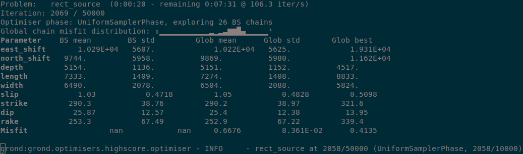
Figure 3: Runtime information given by grond.
Depending on the configured number of iterations and the computer’s hardware the optimisation will run several minutes to hours.
Optimisation report
Once the optimisation is finished we can generate and open the final report with:
grond report -so runs/rect_2009LaAquila.grun
Example report
Explore the online example reports to see what information the inversion reveals.